Autobox Blog

Thoughts, ideas and detailed information on Forecasting.

  • Home
    Home This is where you can find all the blog posts throughout the site.
  • Categories
    Categories Displays a list of categories from this blog.
  • Tags
    Tags Displays a list of tags that has been used in the blog.
  • Bloggers
    Bloggers Search for your favorite blogger from this site.

Forecasting

Subcategories from this category: Uncategorized

You have data that is decreasing.  You have three areas where the data seems to level off.  Is it a trend or is it two level shifts?

If you have any knowledge about what drives the data then by all means use a causal variable.  What to do if you have none?  It then becomes an interesting and very debatable topic.

How many periods determines a level shift might be a big factor here.

Simpson's Paradox is where you have a global significance, but not local.  From a global perspective, sure there is a trend.  From a local, there is no trend. Who is to say that the overall trend will continue?  Who is to say that the trend won't?  Maybe it will go up?


If you run this without making assumptions, you get two level shifts at period 14 and 25 and some outliers using the following data


20324 19856 19012 17247 18616 17786 20509 19097 19437 18562 17648 18672 17324 16765 16108 14742 16567 16041 15511 15403 16797 13977 15570 16249 14005 16645 14098 12310 15923 13422 13030


Y(T) =  18776.                                monthly

+[X1(T)][(-  2800.9    )]        :LEVEL SHIFT      14                                                    2011/ 10

+[X2(T)][(-  2602.3    )]        :LEVEL SHIFT      25                                                    2012/  9

+[X3(T)][(+  3272.0    )]        :PULSE            26                                                    2012/ 10

+[X4(T)][(-  1998.3    )]        :PULSE            22                                                    2012/  6

+[X5(T)][(+  2550.0    )]        :PULSE            29                                                    2013/  1

+                    +   [A(T)]


We were asked to share our thoughts on advantages and disadvantages of forecasting at monthly vs weekly vs daily levels.

Monthly:

Advantages – Fast to compute, easier to model, easier to identify changes in trends, better for strategic long term forecasting


Disadvantages – If you need to plan as the daily level for capacity, people and spoilage of product then higher levels of forecasting won’t help understand the demand on a daily basis as a 1/30th ratio estimate is clearly insufficient.

Causal variables that change on a frequent basis (ie daily/weekly – price, promotion) are not easily integrated into monthly analysis

Integrating Macroeconomic variables like Quarterly Unemployment requires an additional step of creating splines.


Weekly:

Advantages – When you can’t handle the modeling process at a daily level you “settle” for this. When you have very systematic cyclical cycles like “artic ice extents” that follow a rigid curve and not need for day of the week variations.


Disadvantages – Floating Holidays like Thanksgiving, Easter, Ramadan, Chinese New Year change every year and disrupt the estimate for the coefficients for the week of the year impact which CAN be handled by creating a variable for each.

The number of weeks in a year is subject to change and creates a statistical issue due to the fact that every year doesn’t have 52 weeks. We have seen the need to allocate the 53rd week to a “non-player” week to make the data a standard 52 week period which is workable, but disruptive compared to daily data.

Causal variables that change on a frequent basis (ie daily/weekly – price, promotion) are not easily integrated into monthly analysis

Integrating Macroeconomic variables like Quarterly Unemployment requires an additional step of creating splines.


Daily:

Advantages – Weekly data can’t deal with holidays and their lead/lag relationships. If a holiday has days 1,2,3 before the holiday as very large volume a daily model can forecast that while the weekly won’t be able year in and year out model and forecast that impact as the day of the week that the holiday occurs changes every year.

Daily data is superior for short-term/medium tactical forecasting. Days of the week have different patterns which can be identified at this level. Days of the month also can be identified due to pay schedule. Long weekends, Fridays before holidays on Monday, and Mondays following Friday holidays can be identified as important.

Particular weeks of the month may have an identifiable pattern for build up in anticipation for pay schedules. You would want to use daily data as financial forecasting is often quite inaccurate when they employ “ratio estimates”.

It is quicker at reacting to level shifts and changes in trends as the data is being modeled daily vs waiting a week/month to observe the new data. Companies missed the 2008 financial crises as they were not modeling the data at a daily level. The goal is not just forecasting, but also about “early warning” detection of changes in business demand. This detection can be viewed across all lines of business through the use of reporting on level shifts and pulses from a macro view to flag changes.


Disadvantages – Slower to process, but this can be mitigated by reusing models.

Integrating Macroeconomic variables like Quarterly Unemployment requires an additional step of creating splines.


Modeling ARIMA(x) or otherwise known as a Transfer Function models aren't easy to model especially with outliers.  A new book Data Quality for Analytics Using SAS by Gerhard Svolba from SAS shows this to be true.  Click on the link and you will see the graph and the explanation of which outliers were identified.


I am going to make this post short and to the point.

The January 2007 value is an outlier and should have been flagged as one although the author tries to ignore it,  but we do not.

December 2006, January 2008, November 2008, December 2008 are also missed as they are clear outliers.

I will also point out the data seems to be trending up and the forecast is flat, but we don't know what the future values of the causals used so its tough to give a complete view here.

If you have the book and perhaps the data, post it here or send it to us and we will gladly analyze it or any data!

Follow up.....

We downloaded the data and SAS' Universal Viewer. The 4 data sets that they let you download only has transaction level data and it doesn't overlap the time frame for the example. So if the data is not listed in the book, the only way to get it would be to contact the author himself. Here is the author's contact page if anyone wants to do that.

http://support.sas.com/publishing/bbu/companion_site/info.html

We got into an interesting debate on model performance on a classic time series that has been modeled in the famous textbooks and we tried it out on some very expensive statistical software. It's tough to find a journal that is willing to criticize its main advertiser so we will do it for them. The time series is Sales and Advertising and you can even download down below and do this with your own forecasting/modeling tool to see what it does!  Feel free to post your results and continue the debate of what is a good model!

What ingredients are needed in a model?    We have two modeling violations that seem to be ignored in this example:

1)Skipping Identification and "fitting" based on some AIC criteria. Earlier researchers would restrict themselves to lags of y and lags of X and voila they had their model.

2)Ignoring Modern day remedies, but not all do this.  Let's list them out 1)Outliers such as pulses, level shifts, time trends and seasonal pulses.  The historical data seems to exhibit an increasing trend or level shift using just your eyes and the graph. 2)Dealing with too many observations as the model parameters have changed over time(ie Chow test) 3)Dealing with non-constant variance.  These last two don't occur in our example so don't worry about them right now.

Are you (or by default your software) using dated methods to build its regression model?  Is it leaning on the AIC to help build your regression using high order lags?  Said more clearly,  “Are you relying upon using long lags of X in a regression and ignoring using Stochastic (ie ARIMA) or deterministic empirically identified variables to build your model?”   Are you doing this and doing it automatically and potentially missing the point of how to properly model?  Worse yet, do your residuals look like they fail the random (ie N.I.I.D) tests with plots against time?  The annointed D-W statistic can be flawed if there are omitted dummy variables needed such as level shifts, pulses, time trends, or seasonal pulses.  Furthermore, D-W ignores lags 2 and out which ignores the full picture.

See the flow chart on the right hand side on the link in the next sentence. A good model has been tested for necessity and sufficiency. It has also been tested for randomness in the errors.

While it is easy and convenient (and makes for quick run time) to use long lags on X, it can often be insufficient and presumptory (see Model Specification Bias) and leave an artifact in the residuals suggesting an insufficient model.

Regression modelers already know about necessity and sufficiency tests, but users of fancy software don't typically know these important details as to how the system got the model and perhaps a dangerous one?  Necessity tests question whether the coefficients in your model are statistically significant (ie not needed or "stepdown").  Sufficiency tests question whether the model is missing variables and therefore ruled as insufficient(ie need to add more variables or "stepup").

Is it possible for a model to fail both of these two critical tests at the same time?Yes.

Let's look at an example. If we have a model where Y is related to X and previous of values of X up to lag and including lag 4, and lags 2, 3 and 4 are not significant then they should be deleted from the model.  If you don’t remove lag 2, 3 and 4 then you have failed the necessity test and you model is suboptimal.  Sounds like the stepdown step has been bypassed? Yes. The residuals from the “overpopulated” model could(and do!) have pulses and a level shift in the residuals ignored and therefore an insufficient model.

Let’s consider the famous dataset of Sales and Advertising from Blattberg and Jeuland in 1981 that has been enshrined into textbooks like Makradakis, Hyndman and Wheelwright 3rd edition.  See pages 411-413  for this example in the book. The data is 3 years of monthly data.

http://mansci.journal.informs.org/content/27/9/988.full.pdf

Sales - 12,20.5,21,15.5,15.3,23.5,24.5,21.3,23.5,28,24,15.5,17.3,25.3,25,36.5,36.5,29.6,30.5,28,26,21.5,19.7,19,16,20.7,26.5,30.6,32.3,29.5,28.3,31.3,32.2,26.4,23.4,16.4

Adv - 15,16,18,27,21,49,21,22,28,36,40,3,21,29,62,65,46,44,33,62,22,12,24,3,5,14,36,40,49,7,52,65,17,5,17,1

The model in the textbook has 3 lags that are not significant and thereby not sufficient. The errors from the model show the need for AR1 when one is not needed of course due to the fact that there is a poor model being used.  The errors are not random and exhibit a level shift that is not rectified.

In 2013, the largest company that offers statistical software (and very expensive) is seemingly inadequate.  We will withhold the name of this company. The Emperor has no clothes? Nope. She does not. Here is the model in the textbook estimated in Excel (which can be reproduced in Autobox).  The results in the textbook are about the same as this output.  You can clearly see that lags 3,4,5 are NOT SIGNIFICANT, right? Does that bother you?

The residuals are not random and exhibit a level shift in the second half of the data set and two big outliers in the first half not addressed.


Ok, here is the fat and happy expensive forecasting system results (ie "fatted calf" so to speak).  Do you get results like this?  If you did, then you paid too much and got too little.

The MA's 1st parameter was not significant, but kept in the model.  This is indicative of an overparameterized model.  The overloading of coefficients without efficient identification has consequences.


Lack of due diligence - No effort is being made to consider deterministic violations of the error terms.  There are two outliers (one at the beginning and one at the end that are very large (ie 8)) and are not being dealt with which impacts the model/forecast that has been built.

Autobox's turn - Classical remedies have been to add all lags from 0 to N as compared to a smarter approach where only significant variables that also reacts to structure in the errors which could be both stochastic and deterministic.  All the parameters are significant.  Only numerator parameters were needed and no denominator. Note: Stochastic being ARMA structure and deterministic being dummy variables such as pulses, level shifts, time trends and seasonal pulses.

Here are the residuals which are free of pattern.  The last value is ok(ie ~4), but could be confused to be an outlier, but in the end everything is an outlier. :)


If you don’t have the ammunition to examine the errors with a close eye you end up with a model that can fail both necessity and sufficiency at the same time.

Leaning on the AIC leads to ignoring necessity, sufficiency and nonrandom errors and bad models.

Some models in text books show bad models and the keep the modeling approach as simple as possible and are in fact doing damage to the student.  When students become practitioners they find that the text book approach just doesn’t work.


It is the standard Economic Question.  Should I make or build?  The question here is: Should I build my own ARIMA modeling system or use software that can do this automatically? We lay out the general approach how to consider approaches to building a robust model.  Easier said than done does apply here.


Overview

Autoregressive Integrated Moving Average (ARIMA) is a process designed to identify a weighted moving-average model specifically tailored to the individual dataset by using time series data to identify a suitable model. It is a rear-window approach that doesn’t use user-specified helping variables; such as price and promotion.  It uses correlations within the history to identify patterns that can be statistically tested and then used to forecast.  Often we are limited to using only the history and no causals whereas the general class of Box-Jenkins models can efficiently incorporate causal/exogenous variables (Transfer Functions or ARIMAX).

This post will introduce the steps and concepts used to identify the model, estimate the model, and perform diagnostic checking to revise the model. We will also list the assumptions and how to incorporate remedies when faced with potential violations.


Background

Our understanding of how to build an ARIMA model has grown since it was introduced in 1976 (1).  Properly formed ARIMA models are a general class that includes all well-known models except some state space and multiplicative Holt-Winters models. As originally formulated, classical ARIMA modeling attempted to capture stochastic structure in the data; little was done about incorporating deterministic structure other than a possible constant and/or identifying change points in parameters or error variance.

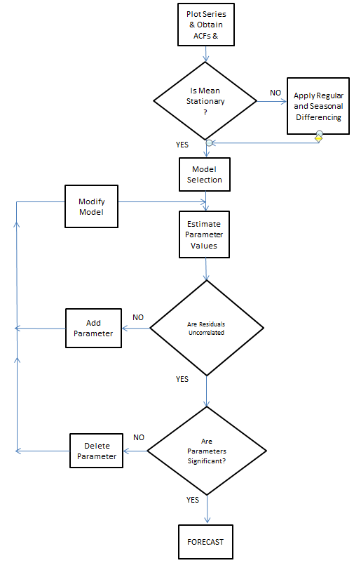
We will highlight procedures relevant to suggested augmentation strategies that were not part of the original ARIMA approach suggested in but are now standard. This step is often ignored as it is necessary that the mean of the residuals is invariant over time and that the variance of the final model’s errors is constant over time.  Here is the classic circa 1970.


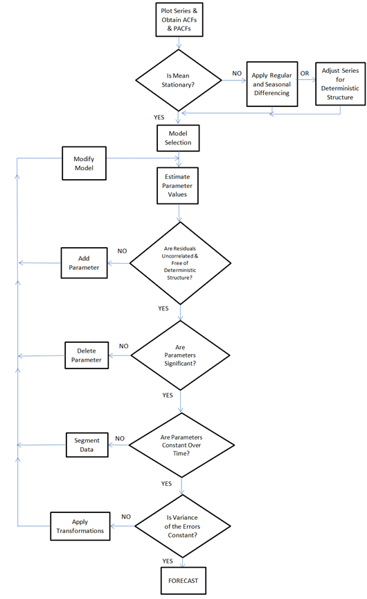
Here is the flowchart revised for additions by Tsay, Tiao, Bell, Reilly & Gregory Chow (ie chow test)


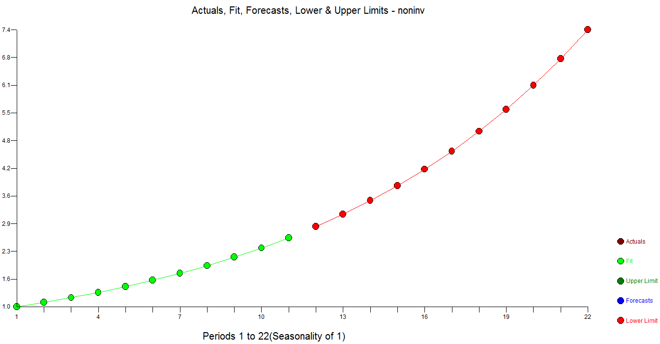
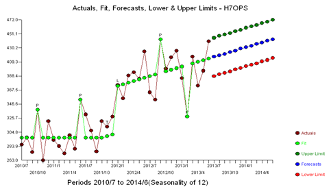
The idea of modeling is to characterize the pattern in the data and the goal is to identify an underlying model that is generating and influencing that pattern.   The model that you will build should match the history which can then be extrapolated into the future.  The actual minus the fitted values are called the residuals.  The residuals should be random around zero (i.e. Gaussian) signifying that the pattern has been captured by the model.


For example, an AR model for monthly data may contain information from lag 12, lag 24, etc.

i.e. Yt = A1Yt-12 +A2 Yt-24  + at

This is referred to as an ARIMA(0,0,0)x(2,0,0)12 model
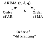
General form is ARIMA(p,d,q)x(ps,ds,qs)s


Tools


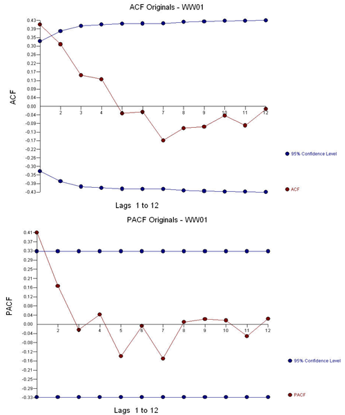
The ARIMA process uses regression/correlation statistics to identify the stochastic patterns in the data.  Regressions are run to find correlations based on different lags in the data. The correlation between successive months would be the lag 1 correlation or in ARIMA terms, the ACF of lag 1. We then examine if this month is related to one year ago at this time would then be apparent from evaluating the lag 12 correlation or in ARIMA terms, the ACF of lag 12. By studying the autocorrelations in the history, we can determine if there are any relationships and then take action by adding parameters to the model to account for that relationship. The different autocorrelations for the different lags are arranged together in what is known as a correlogram and are often presented using a plot. They are sometimes presented as a bar chart.  We present it as a line chart showing 95% confidence limits around 0.0. The autocorrelation is referred to as the autocorrelation function (ACF).

  • The key statistic in time series analysis is the autocorrelation coefficient (the correlation of the time series with itself, lagged 1, 2, or more periods).

The Partial Autocorrelation Function (PACF).  The PACF of lag 12 for example is a regression using a lag of 12, but also uses all of the lags from 1 to 11 as well, hence the name partial. It is complex to compute and we won’t bother with that here.

Now that we have explained the ACF and the PACF, let’s discuss the components of ARIMA.  There are three pieces to the model. The “I” means Integrated, but it simply means that you took differencing on the Y variable during the modeling process. The “AR” means that you have a model parameter that explicitly uses the history of the series.  The “MA” means that you have a model parameter that explicitly uses the previous forecast errors. Not all models have all parts of the ARIMA model. All models can be re-expressed as pure AR models or pure MA models. The reason we attempt to mix and match has to do with attempting to use as few parameters as possible.

Identifying the order of differencing starts with the following initial assumptions, which are ultimately need to be verified:

1) The sequence of errors (a’s) are assumed to have a constant mean of zero and a constant variance for all sub-intervals of time.

2) The sequence of errors (a’s) are assumed to be normally distributed where the a’s are independent of each other.

3) Finally the model parameters and error variance are assumed to be fixed over all sub-intervals.


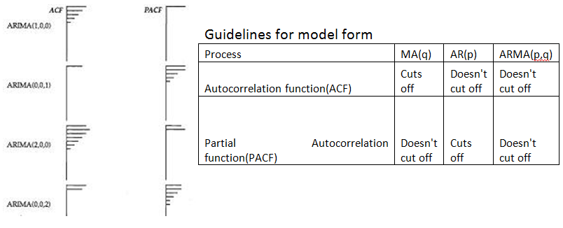
We study the ACF and PACF and identify an initial model. If this initial model is significant, the residuals will be free of structure and we are done. If not, we identify that structure and add it to the current model until a subsequent set of residuals is free of structure. One could consider this iterative approach as moving structure currently in the errors to the model until there is no structure in the errors to relocate.


The following are some simplified guidelines to apply when identifying an appropriate ARIMA model with the following assumptions:

Guideline 1: If the series has a large number of positive autocorrelations then differencing should be introduced. The order of the differencing is suggested by the significant spikes in the PACF based upon the standard deviation of the differenced series. This needs to be tempered with the understanding that a series with a mean change or a trend change can also have these characteristics.

Guideline 2: Include a constant if your model has no differencing; include a constant elsewhere if it is statistically significant.

Guideline 3: Domination of the ACF over the PACF suggests an AR model while the reverse suggests an MA model. The order of the model is suggested by the number of significant values in the subordinate.

Guideline 4: Parsimony: Keep the model as simple as you can, but not too simple as overpopulation often leads to redundant structure.

Guideline 5: Evaluate the statistical properties of the residual (at) series and identify the additional structure (step-forward) required

Guideline 6: Reduce the model via step-down procedures to end up with a minimally sufficient model that has effectively deconstructed the original series to signal and noise. Over-differencing leads to unnecessary MA structure while under-differencing leads to overly complicated AR structure.


If a tentative model exhibits errors that have a mean change this can be remedied in a number of ways;


1) Identify the need to validate that the errors have constant mean via Intervention Detection (2,3) yielding pulse, seasonal pulse/level shift/local time trends

2) Confirming that the parameters of the model are constant over time

3) Confirming that the error variance has had no deterministic change points or stochastic change points.


The tool to identify omitted deterministic structure is fully explained in references 2 and 3 as follows:

1) use the model to generate residuals

2) identify the intervention variable needed following the procedure defined in reference

3) Re-estimate the residuals incorporating the effect into the model and then go back to Step 1 until no additional interventions are found.


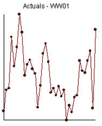
Example 1) 36 annual values:

The ACF and the PACF suggest an AR(1) model (1,0,0)(0,0,0).


Leading to an estimated model (1,0,0)(0,0,0).

With the following residual plot, suggesting some “unusual values”:


The ACF and PACF of the residuals suggests no stochastic structure as the anomalies effectively downward bias the results:


We added pulse outliers to create a more robust estimate of the ARIMA coefficients:

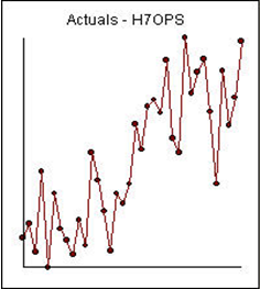
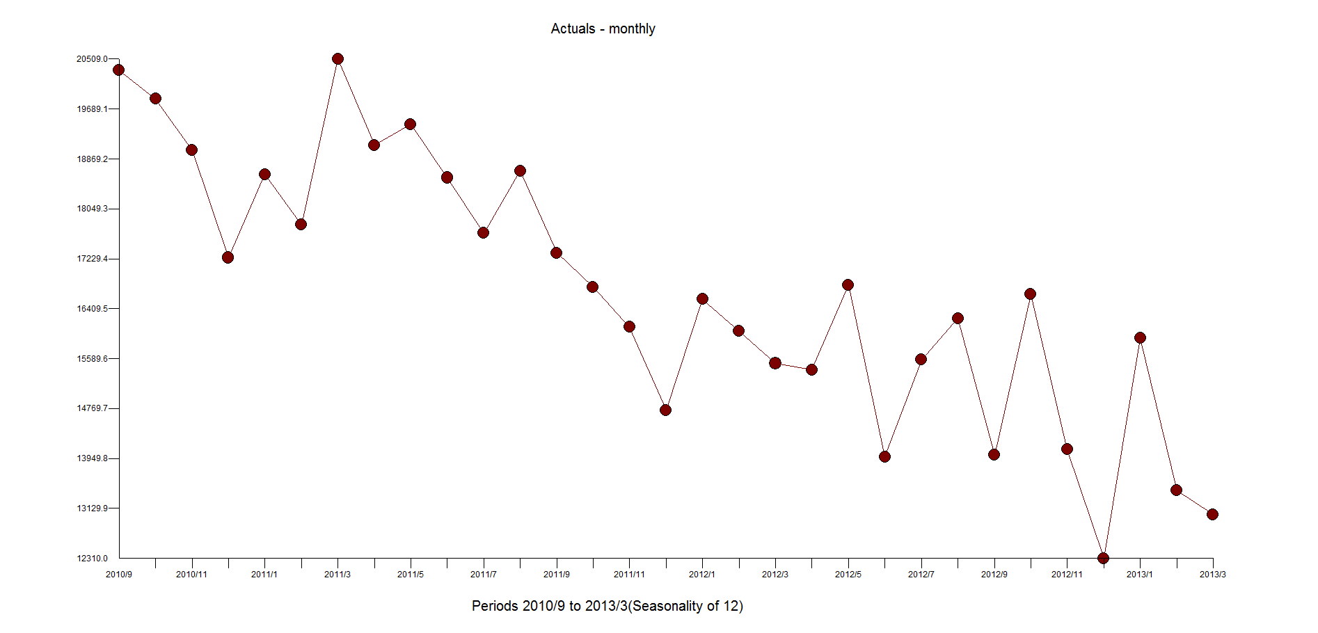
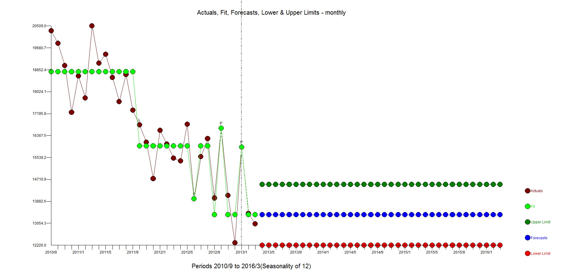
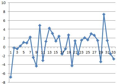
Example 2) 36 monthly observations:


With ACF and PACF:


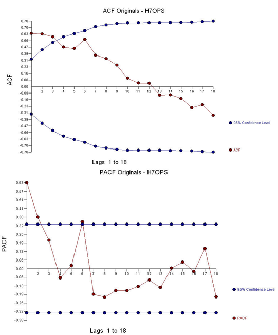
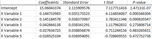
Leading to an estimated model:  AR(2) (2,0,0)(0,0,0)


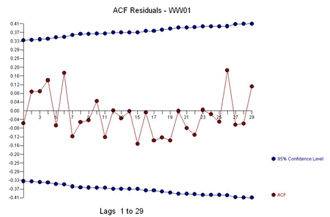
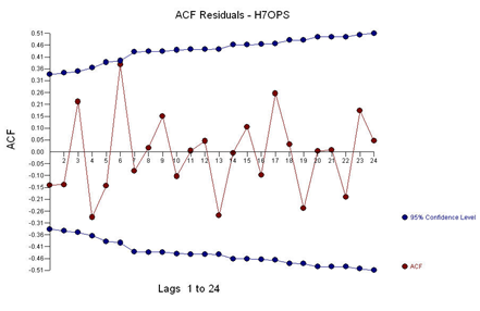
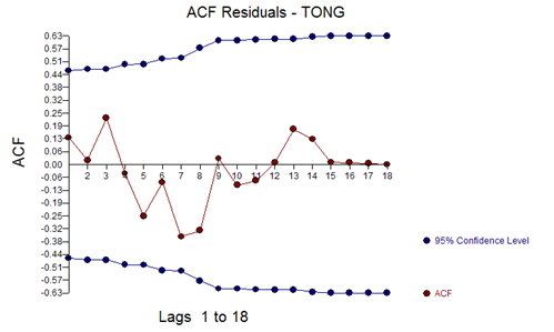
And with ACF of the residuals:


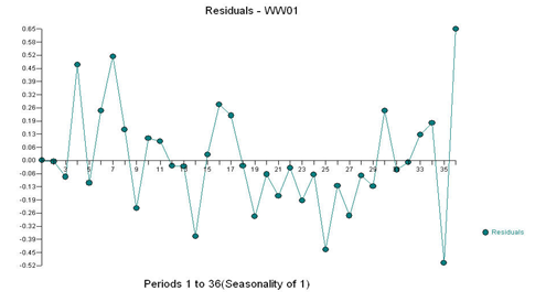
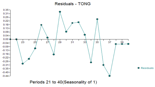
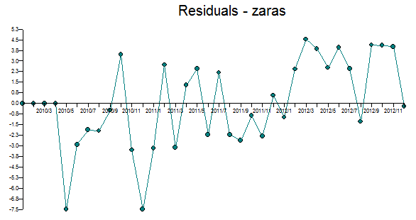
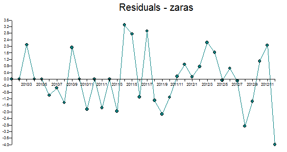
With the following residual plot:


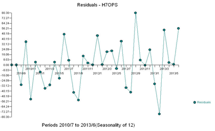
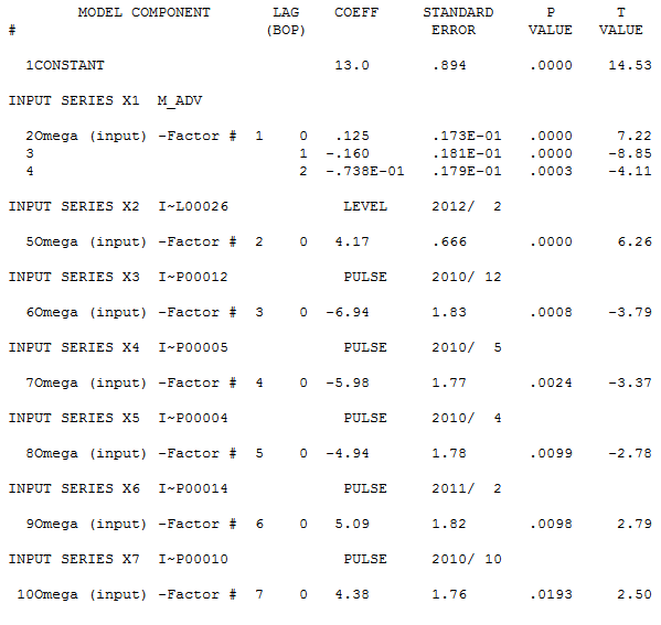
This example is a series that is better modeled with a step/level shift.

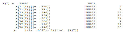
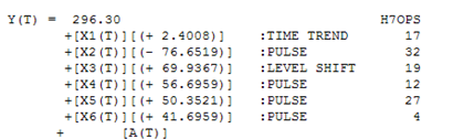
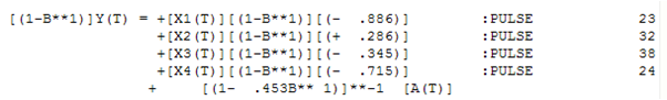
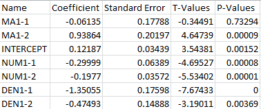
The plot of the residuals suggests a mean shift. Empowering Intervention Detection leads to an augmented model incorporating a level shift and a local time trend with and 4 pulses and a level shift. This model is as follows:


Example 3) 40 annual values:


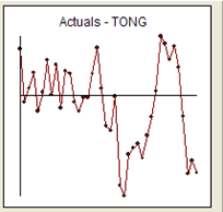
The ACF and PACF of the original series are:


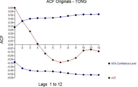
Suggesting a model (1,0,0,(0,0,0)


With a residual ACF of:
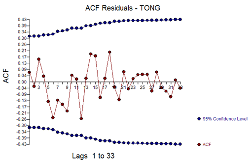


And residual plot:


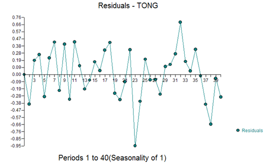
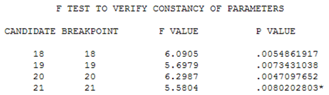
This suggests a change in the distribution of residuals in the second half of the time series.  When the parameters were tested for constancy over time using the Chow Test (5), a significant difference was detected at period 21.


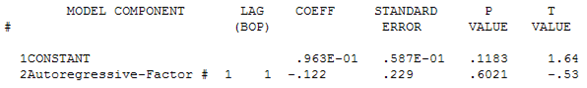
The model for period 1-20 is:


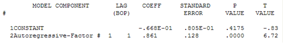
The model for period 21-40 is:


A final model using the last 20 values was:


With residual ACF of:


And residual plot of:


References

1)Box, G.E.P., and Jenkins, G.M. (1976). Time Series Analysis: Forecasting and Control, 2nd ed. San Francisco: Holden Day.

2)Chang, I., and Tiao, G.C. (1983). "Estimation of Time Series Parameters in the Presence of Outliers," Technical Report #8, Statistics Research Center, Graduate School of Business, University of Chicago, Chicago.

3)Tsay, R.S. (1986). "Time Series Model Specification in the Presence of Outliers," Journal of the American Statistical Society, Vol. 81, pp. 132-141.

4)Wei, W. (1989). Time Series Analysis Univariate and Multivariate Methods. Redwood City: Addison Wesley.

5)Chow, Gregory C. (1960). "Tests of Equality Between Sets of Coefficients in Two Linear Regressions". Econometrica 28 (3): 591–605


Everyone is asked this question.

Everyone tries to answer it.

Everyone wants the "Early Warning" and quarter end numbers for "the street".  Finance or Accounting are often asked by the organization to make these projections, but the truth is (and hurts) that they don't have the time series analysis tools and awareness needed to provide a good forecast.

The question is "Are you using your modeling skills to help you answer that question" or are you using simple averaging and ratio estimates to figure this one out?

We were asked at a Forecasting Conference by a P&G employee how to do this.  They had NOT identified the change in level down due to the financial crises in 2008.  Why? They were using simple approaches to forecast to a not so simple problem.  You need to model the data to do it correctly and not just blindly apply back of the envelope methods.

The problem is that when you use simple methods like ratio estimates you are assuming that Wednesday's behave the same as Saturdays. That assumption is the problem.  Less likely, but often we see the first few days of the month stronger due to a paycheck effect. So, the first few days are an outlier and yet they are being used to project. The wrong way to forecast the month end number is like this:

We are 5 days into the month and we want to forecast the expected month end number.  We take the first 5 days revenue/sales(ie $47,000).  We take the number of days in a month (ie 30) and take 30 and divide it by 5 which results in a factor of 6.  We multiply 6 by the 5 days of revenue and that is the forecast.  $47,000*6=$282,000.


The report you should be getting from your statistical software should look like this.  It provides a table of forecasts and the probability of making different numbers.    This allows you to interpolate your target number to find out where you stand using statistics and not simplistic division and multiplication.  Different levels of statistical confidence are set and the history plus the forecast are aggregated to provide a month end number.  The expected forecast is the 50% confidence level.


PROBABILITY FORECAST


99.862335 17521950.24


99.740551 17804768.87


99.528383 18087587.5


99.172964 18370406.13


98.600522 18653224.75


97.714171 18936043.38


96.394897 19218862.01


94.507447 19501680.64


91.911957 19784499.27


88.481731 20067317.9


84.124939 20350136.53


78.806855 20632955.15


72.569247 20915773.78


65.538755 21198592.41


57.924343 21481411.04


57.924343 21481411.04


50 21764229.67


42.075657 22047048.3


34.461245 22329866.93


27.430753 22612685.56


21.193145 22895504.18


15.875062 23178322.81


11.518269 23461141.44


8.088043 23743960.07


5.492553 24026778.7


3.605103 24309597.33


2.285829 24592415.96


1.399478 24875234.59


0.827036 25158053.21


0.471617 25440871.84


0.259449 25723690.47


0.137665 26006509.1


To do this properly, you need to model the data using daily data.  We recommend about 3 years of historical data.  You need to consider all of these issues:

Day of the week effects, Seasonality, Trends, Holiday effects, Day of the month effects, outliers, Lead/Lags around Holidays, changes in seasonality(ie Saturdays are high and then over time becomes like the other days of the week)

Once you build a model that is sophisticated to truly model and understand the patterns within the data, you can then forecast with a reduced level of bias.  Let's describe SOME of the different components in this model now

1)The average demand is 148k 2)Demand is low by 241k on Women's Day - note that this is data from South Africa 3)The day before Reconciliation Day is high by 113k 4)MONTH_EFF09 means Septembers are typically low by 11k 5)FIXED_EFF_N10107 means that the first day of the week is low by 164k Note that the data begins on 7/1/2007 which is a Sunday 6)WKINM01 means that the first week of the month is high by 64k 7)FIXED_DAY01 means that the first day of the month is low by 56k 8)SEASONAL PULSE beginning at  164/ 2 8/16/2010 means that volume AT or ABOUT on Mondays became higher by 152k starting on 8/16/2010 9)LEVEL SHIFT beginning at 7/30/2010 found overall volume to be higher by 21k. 10)PULSE outlier found on 11/1/2010 was low by 368k.  The 41 outliers are reported by importance statistically.


Series __07010796RRAE

Y(T) =  .14855E+06                                                                                     
       +[X1(T)][(-  .24148E+06)]                                       G_WOMEN
       +[X2(T)][(-  .18020E+06)]                                       G_HERITAGE
       +[X3(T)][(+  .11308E+06B**-1-  .25778E+06+  .18230E+06B** 1                                                      
       +  .23546E+06B** 2+  .19179E+06B** 3+  .18266E+06B** 5)]        G_RECONCILE
       +[X4(T)][(+  .16671E+06B**-3+  .17821E+06B**-2+  .15050E+06B**-1                                                 
       -  .22621E+06-  .19222E+06B** 1)]                               M_XMAS
       +[X5(T)][(+  .31591E+06B**-4+  .17758E+06B**-3+  64947.    B**-2                                                 
       -  .21378E+06)]                                                 M_NEWYEARS
       +[X6(T)][(-  72258.    B**-3-  .20193E+06B**-2+  87829.    B**-1                                                 
       -  .20174E+06B** 1)]                                            M_EASTER
       +[X7(T)][(-  .23159E+06+  94924.    B** 1)]                     G_FREEDOM
       +[X8(T)][(+  90703.    B**-2+  49047.    B**-1-  .18390E+06)]   G_WORKERS
       +[X9(T)][(-  .23416E+06+  51151.    B** 1+  76470.    B** 2)]   G_YOUTH
       +[X10(T)[(-  11845.    )]                                       MONTH_EFF09
       +[X11(T)[(-  21861.    )]                                       MONTH_EFF10
       +[X12(T)[(-  17001.    )]                                       MONTH_EFF11
       +[X13(T)[(-  20620.    )]                                       MONTH_EFF01
       +[X14(T)[(-  29782.    )]                                       MONTH_EFF02
       +[X15(T)[(-  13982.    )]                                       MONTH_EFF03
       +[X16(T)[(-  11262.    )]                                       MONTH_EFF04
       +[X17(T)[(-  .16496E+06)]                                       FIXED_EFF_N10107
       +[X18(T)[(+  .13591E+06)]                                       FIXED_EFF_N10307
       +[X19(T)[(+  87981.    )]                                       FIXED_EFF_N10407
       +[X20(T)[(+  38655.    )]                                       FIXED_EFF_N10507
       +[X21(T)[(+  25474.    )]                                       FIXED_EFF_N10607
       +[X22(T)[(+  64857.    )]                                       WKINM01
       +[X23(T)[(-  56641.    )]                                       FIXED_DAY01
       +[X24(T)[(+  46855.    )]                                       FIXED_DAY08
       +[X25(T)[(+  44857.    )]                                       FIXED_DAY09
       +[X26(T)[(+  22607.    )]                                       FIXED_DAY10
       +[X27(T)[(+  17102.    )]                                       FIXED_DAY17
       +[X28(T)[(+  .15233E+06)]                                       :SEASONAL PULSE 1143                164/  2   8/16/2010   I~S01143__07010796RRAE
       +[X29(T)[(+  21070.    )]                                       :LEVEL SHIFT    1126                      161/  6   7/30/2010   I~L01126__07010796RRAE
       +[X30(T)[(-  .36860E+06)]                                       :PULSE          1220                      175/  2  11/ 1/2010   I~P01220__07010796RRAE
       +[X31(T)[(-  .37728E+06)]                                       :PULSE           170                       25/  2  12/17/2007   I~P00170__07010796RRAE
       +[X32(T)[(-  32079.    )]                                       :LEVEL SHIFT     417                       60/  4   8/20/2008   I~L00417__07010796RRAE
       +[X33(T)[(-  .29897E+06)]                                       :PULSE          1067                      153/  3   6/ 1/2010   I~P01067__07010796RRAE
       +[X34(T)[(+  29329.    )]                                       :LEVEL SHIFT     139                       20/  6  11/16/2007   I~L00139__07010796RRAE
       +[X35(T)[(-  .28982E+06)]                                       :PULSE          1129                      162/  2   8/ 2/2010   I~P01129__07010796RRAE
       +[X36(T)[(+  .19134E+06)]                                       :PULSE           536                       77/  4  12/17/2008   I~P00536__07010796RRAE
       +[X37(T)[(-  .26880E+06)]                                       :PULSE          1038                      149/  2   5/ 3/2010   I~P01038__07010796RRAE
       +[X38(T)[(-  .22253E+06)]                                       :PULSE           662                       95/  4   4/22/2009   I~P00662__07010796RRAE
       +[X39(T)[(-  .26024E+06)]                                       :PULSE          1159                      166/  4   9/ 1/2010   I~P01159__07010796RRAE
       +[X40(T)[(-  .29674E+06)]                                       :PULSE           547                       79/  1  12/28/2008   I~P00547__07010796RRAE
       +[X41(T)[(-  .30180E+06)]                                       :PULSE           171                       25/  3  12/18/2007   I~P00171__07010796RRAE
       +[X42(T)[(-  .26154E+06)]                                       :PULSE           303                       44/  2   4/28/2008   I~P00303__07010796RRAE
       +[X43(T)[(+  .17179E+06)]                                       :PULSE           308                       44/  7   5/ 3/2008   I~P00308__07010796RRAE
       +[X44(T)[(+  .21111E+06)]                                       :PULSE           180                       26/  5  12/27/2007   I~P00180__07010796RRAE
       +[X45(T)[(+  .24487E+06)]                                       :PULSE           169                       25/  1  12/16/2007   I~P00169__07010796RRAE
       +[X46(T)[(-  .20171E+06)]                                       :PULSE          1097                      157/  5   7/ 1/2010   I~P01097__07010796RRAE
       +[X47(T)[(+  .28926E+06)]                                       :PULSE           173                       25/  5  12/20/2007   I~P00173__07010796RRAE
       +[X48(T)[(+  .18024E+06)]                                       :PULSE          1139                      163/  5   8/12/2010   I~P01139__07010796RRAE
       +[X49(T)[(-  .21759E+06)]                                       :PULSE           772                      111/  2   8/10/2009   I~P00772__07010796RRAE
       +[X50(T)[(+  .22993E+06)]                                       :PULSE           302                       44/  1   4/27/2008   I~P00302__07010796RRAE
       +[X51(T)[(-  .26803E+06)]                                       :PULSE           307                       44/  6   5/ 2/2008   I~P00307__07010796RRAE
       +[X52(T)[(-  15373.    )]                                       :SEASONAL PULSE  833                      119/  7  10/10/2009   I~S00833__07010796RRAE
       +[X53(T)[(-  .18772E+06)]                                       :PULSE          1189                      170/  6  10/ 1/2010   I~P01189__07010796RRAE
       +[X54(T)[(+  .21572E+06)]                                       :PULSE           771                      111/  1   8/ 9/2009   I~P00771__07010796RRAE
       +[X55(T)[(+  9024.5    )]                                       :LEVEL SHIFT     901                      129/  5  12/17/2009   I~L00901__07010796RRAE
       +[X56(T)[(+  97577.    )]                                       :PULSE           367                       53/  3   7/ 1/2008   I~P00367__07010796RRAE
       +[X57(T)[(+  .17982E+06)]                                       :PULSE           182                       26/  7  12/29/2007   I~P00182__07010796RRAE
       +[X58(T)[(+  .12688E+06)]                                       :PULSE           312                       45/  4   5/ 7/2008   I~P00312__07010796RRAE
       +[X59(T)[(+  .13894E+06)]                                       :PULSE           313                       45/  5   5/ 8/2008   I~P00313__07010796RRAE
       +[X60(T)[(+  .14256E+06)]                                       :PULSE          1040                      149/  4   5/ 5/2010   I~P01040__07010796RRAE
       +[X61(T)[(+  .13974E+06)]                                       :PULSE           408                       59/  2   8/11/2008   I~P00408__07010796RRAE
       +[X62(T)[(-  .19002E+06)]                                       :PULSE           996                      143/  2   3/22/2010   I~P00996__07010796RRAE
       +[X63(T)[(+  49165.    )]                                       :SEASONAL PULSE  632                       91/  2   3/23/2009   I~S00632__07010796RRAE
       +[X64(T)[(+  29613.    )]                                       :SEASONAL PULSE 1088                      156/  3   6/22/2010   I~S01088__07010796RRAE
       +[X65(T)[(+  .14847E+06)]                                       :PULSE          1013                      145/  5   4/ 8/2010   I~P01013__07010796RRAE
       +[X66(T)[(+  .12300E+06)]                                       :PULSE           270                       39/  4   3/26/2008   I~P00270__07010796RRAE
       +[X67(T)[(-  .16349E+06)]                                       :PULSE           540                       78/  1  12/21/2008   I~P00540__07010796RRAE
       +[X68(T)[(-  .19112E+06)]                                       :PULSE           176                       26/  1  12/23/2007   I~P00176__07010796RRAE
      +                    +   [A(T)]

This looks easy to do, right?


You were taught and told through books, teachers, websites and your software that your AR model coefficient can't be outside the -1 to +1 region. This is also often stated as that "unit root" needs to be outside the unit circle, but this just isn't true. A criticism of Box-Jenkins modeling was that it wasn't applicable to growth models.

Ok, but why does that matter to me? Well, it matters to you as that means you have been operating under an assumption that limits your modeling to handle explosive data from perhaps a product launch where sales really take off. Typically, the long run forecasts from such a time series are not usually realistic, but the mid to short are useful.

Let's look at annual data that has explosive and "multiplicative" growth.

1.1 1.21 1.33 1.46 1.61 1.77 1.95 2.14 2.36 2.59   <<<<<----------  Note how the incremental differences keep getting larger(ie .11, .12, .13, .15, .16, .18, .19, .22, .23)

If we modeled this based on what we were taught or using a typical forecasting tool, it would build a model with double differencing and an AR 1. The forecasts The residuals would show that the model didn't actually capture the signal as it was constrained by the bounds of the unit circle(-1 to +1).

ARIMA(1,2,0) Coefficients: ar1 0.6868 s.e. 0.2121 sigma^2 estimated as 0.0001214: log likelihood=27.48 AIC=-50.97 AICc=-48.97 BIC=-50.57

Below are the forecasts.  Note the almost flat forecast and lack of explosive growth.

2.84 3.1 3.37 3.64 3.92 4.2 4.48 4.76 5.04 5.32 5.6   <<<<<----------   Note how the incremental differences are not growing like they should. (ie .26, .26, .27, .28, .28, .28, .28, .28)


Most software and people ignore the residual plot.  This is a big mistake.  This is a clear way of checking to see if the model was built in a robust manner by checking if the residuals are random or also known as Normal Independently Identically Distributed (N.I.I.D.) which is the ASSUMPTION that the whole modeling process is built upon, but again ignored.  The residuals are not random at all.


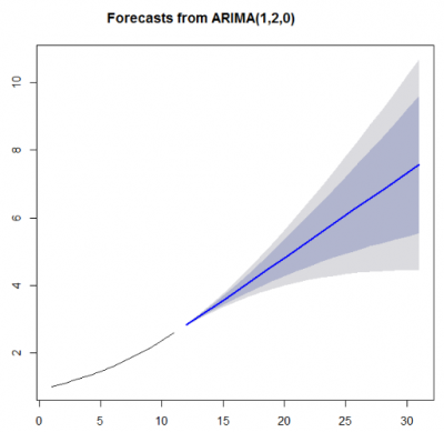
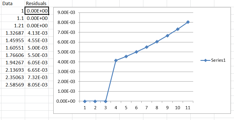
If we ignore the unneeded unit circle constraint,  the model would be again double differencing with an AR1 coefficient that is 1.1 and very much OUTSIDE the unit circle and very estimable!

[(1-B**1)][(1-B**1)]Y(T) = .82601E-07 + [(1- 1.1000B** 1)]**-1 [A(T)]


Posted by on in Forecasting


Moving away from Allocation of Historical Contributions to Multiple Regression Models

Allocation vs. Modeling

Today’s approaches to forecasting for example, inbound call center volume, rely upon calculating “contributions” from historical data and then allocating those to create a forecast using Excel or some similarly with programming code in SAS or R.  For example, you might take the last year of data and calculate the total and find out that January “contributed” 1% to the total year and then use that to help forecast next January.  The guiding assumption is that the distributions are constant and don’t change.   For the day of the week forecast, using the same type of approach looking at how the 7 days of the week percentages stack up over the last year.  If we wanted to forecast 16 semi-hours of the day, we would identify and allocate percentages.  We could identify an average impact of holidays on and around and also an average impact of long weekends that are used inappropriately for all holidays.  These percentage based allocations don’t account for the nuances in the data that need to be addressed in order to have a high quality forecast.  These approaches could be enhanced using statistical modeling techniques called as multiple regression that will identify complexities in the data.  Multiple regression will attempt to do similar things like we just discussed, but allow for many more complicated issues that occur.  For example, outliers occur in data and if ignored will skew the forecast and can be identified and adjusted for using schemes to search and detect.  See Ruey Tsay’s Work on Outlier detection for more on this. Additionally, if there are changes in trends(up or down) in the data that need to be factored  with a trend variable and yes there could be more than one trend!  There could be changes in the mean that are not a trend, but more of a one-time bump (ie level shift) and yes again there could be more than one level shift! Your marketing promotions might be the reason for the level shift, but if you don’t actually model that promotion statistically you aren’t going to be able to leverage it into the forecast like you can do with regression modeling.  There could be changes over time where Mondays were always low and now become high (ie seasonal pulse). You will have single one time “pulse” outliers that need to be adjusted for as random swings occur without cause.  Now, you might be aware of some of these outliers like system outages and you should include them as a dummy causal variable to explain the variability caused by it.  Economists call this knowledge “apriori” when building these models. If you don’t have a forecasting approach that identifies these changes then your forecast will ignore all of these impacts and you will be left with a poor man’s modeling approach or what accountants like to call “allocation”.

Some try and model the call volume data and other data on a weekly level.  Weekly level data is severely impacted by moving holidays like Easter, Thanksgiving and Ramadan.  In addition, using weekly level data means that you are allocating and not modeling your data.  You should also know that all of the items listed in the previous paragraph can’t be factored into the forecast using weekly data.

We know:

Different days in a week have statistically different call patterns

Different semi-hours in a day have statistically different call patterns based on which day of the week it is


How do we solve this problem? Mixed Frequency Modeling

To solve all of the above, this approach can be best described as “Mixed Frequency”.  It is called Mixed Frequency because the seasonality of the two datasets that will be analyzed are different but used together.  The daily level data is a seasonality of 7.  The semi-hourly data is a seasonality of 48.

STEP 1 :To solve this puzzle, we build a regression model at the daily level using promotional variables(lead and lag impacts) and the future expected promotions, 16 U.S. holidays(lead and lag impacts), days of the week with 6 dummy variables, search for special days of the month, months of the year, impact on Mondays after holiday, impact on Fridays before a holiday, along with checking for changes in trend, level shifts, outliers and seasonal pulses to get a forecast.  We recommend 3 years of historical data so that you can get a good measure on the holidays.  For example, in 2010 and 2011 Christmas landed on a weekend so you have no measure of the impact of Christmas on a weekday.  You could include a causal that explains the macro direction of the business (ie # of outlets your product is sold in) always be used as a good causal to help explain the overall trend in the call volume.  You could provide future sales estimates using a forecast to help guide the direction of the forecast as well as allow the managements input on expected future business success for upcoming months.

STEP 2: If you wanted to forecast the 9 am to 5 pm time frame by half hour periods, you would use the history and forecast from or the daily level data and use it as causal.  You would use that causal in each of 16 separate regressions for each of the half hour data sets.  The daily causal and the day of the week causal would be forced into the model so as to provide a “guiding hand” for each of the semi-hours. This framework allows the day of the week and intraday nuances to be modeled and forecasted.

The Forecasts from the first step building the “daily level” model and forecast would need to go through a “Forecast Reconciliation” step so that the sum of the 16 semi-hourly forecasts would match the daily level.  The opposite could be done if requested.

Try challenging your vendor or your forecaster and ask them how they actually calculate the forecast.    Are they allocating or modeling?


Does free software do what you thought it would?

For ANOVA and t-tests, the R packages are just fine as this type of statistics is pretty basic with not a lot of moving parts, but when you are trying to model time series data or to do pattern recognition with that data is much much more difficult.

Is there "version" control with the R software packages?  Yes, there seems to be.  Errors are documented and tracked in the Change log section.  Take a good close look at this log and the number of changes and the changes made.

Statistical forecasting software has been found to have different forecasts for the identical model and different estimates of the parameters.  Bruce McCullough from Drexel University has spent a large part of his statistical career publishing journal articles that debunk forecasting software and their errors.  Bruce first railed on Excel's inability to be trusted as a reliable source for statistics.  Others have taken up that same cause with Google's Spreadsheets.

A paper by Yalta showed problems with ARIMA modeling benchmarks in some packages and showing Autobox, GRETL, RATS, X-12-ARIMA to be correctly estimating models.  The references at the bottom of that paper show the main papers in this area of research, if you are interested.  Many of them McCullough's.

At a recent meeting with customers and prospects, the topic of whether R packages could be used for Corporate analysis came up.  We can tell you that it is being used for Corporate and personal and Dissertations and on and on.  We shared our experience with someone testing out the auto.arima forecasting package which had a model which was flawed.  Models are debatable for sure, but having "buggy" software is not just acceptable for a business or even research environment as bad forecasting has bad consequences. We would like to help you in your evaluation of your models. One way for you to do this is to take the residuals from your forecasting software model and enter it into a trial version of AUTOBOX (http://www.autobox.com/cms/index.php/30day). If AUTOBOX finds a model, other than a constant, then you can conclude that your model missed a piece of information and that you chose wrong with your current tool. Sometimes software is worth what you pay for it.

Most software has releases every year or every other year.  Extensive testing is performed on benchmarks to identify errors and prove that the software is stable.  Most software uses Regression testing to identify and correct for issues.  If a version gets created every other month or week can you trust it to run your Enterprise or even Dissertation?


15 Questions surrounding outliers and time series forecasting/modeling


Does your current forecasting process automatically adjust for outliers? (correct answer Yes)

Do you make a separate run for certain problems that SHOULD NOT get adjusted for outliers as the outliers are in fact real and shouldn't be adjusted?  (correct answer Yes)

Do you know what standard deviations are used to identify an outlier?  (correct answer "who cares" You shouldn't be having to tell the system)

Who knows that the standard deviation calculation is itself skewed by the outlier?  (correct answer "who cares" You shouldn't be having to tell the system)

Does the system ask you how many times it should "iterate" when removing outliers? How many times do you "iterate"? (correct answer "who cares" You shouldn't be having to tell the system)

Does the system allow you to convert outliers to causals and flag future values when the event will happen again?  (correct answer Yes)

Does the system identify inliers? ie. 1,9,1,9,1,9,1,5  (correct answer Yes)

Does the system recognize the difference between an outlier and a seasonal pulse?  (correct answer Yes) (IE 1,0,0,0,0,0,0,0,0,0,0,0,1,0,0,0,0,0,0,0,0,0,0,0,1,0,etc)

Does the system recognize the difference between an outlier and a level shift?  (correct answer Yes) (IE 0,0,0,0,0,0,0,0,0,0,1,1,1,1,1,1,1,1,1,1,etc)

Does the system recognize the difference between an outlier and a change in the trend?  (correct answer Yes)  (IE 0,0,0,0,0,0,0,1,2,3,4,5,6,7,8,etc)

Does the system allow you to force the outlier in the most recent period to be a "level shift" or a "seasonal pulse"?  (correct answer Yes)

Does the system report a file adjusted for outliers for pure data cleansing purposes?  (correct answer Yes)

Does the system adjust for outliers in a time series regresion (ie ARIMAX/Transfer Function)? (correct answer Yes)

Who tries to find the assignable cause why the outliers existed?   (correct answer I do)

Who then provides causals to explain the outliers to the system?   (correct answer I do)

Posted by on in Forecasting

In June 2012, Rob Hyndman moved his database of famous time series to Datamarket.com

You can access these classic and very good examples to do bench marking on software here.

The M3 competition data can be gotten from here.


Exploiting the Value of Information

Don’t tell me I can look anywhere in the database.  Tell me where to look for something I didn’t know.

  • Have we detected a common systematic patterns amongst many SKUs where certain SKUs seem to be exhibiting similar unusual patterns as discussed in the next 3 bullets:
  • Have we detected a statistically significant change in the most recent observation in our time series?
  • Have we detected a statistically significant change in the trend in our time series?
  • Have we detected a statistically significant change in the average(ie level shift) in our time series?

Do I need to plan using daily data?

  • Are days of the week unusual?
  • Are there particular days in the month unusual?
  • Is the Monday after a holiday or Friday before a holiday unusual?
  • Have we detected a statistically significant change in the seasonal factors(ie day of the week impact) in our time series?
  • Will we make the month end number?  It is 10 days into the month. Most use a overly simple ratio estimate when they should be using daily data to model and forecast the probability that we are going to exceed the plan/goal number for the month.

I need to know when we will reach our capacity.  When in the future will we exceed a user-specified high-side critical value and precisely when is this expected to happen with a confidence level?

Have we detected a statistically significant change in variability?

Have we detected a statistically significant change in the model such that the older data needs to be truncated as the pattern has completely changed?

What can we expect to happen if we alter our advertising/promotion/price activity?


Matt presented his results at the ISF(http://www.forecasters.org and his presentation is here http://www.forecasters.org/proceedings12/WELLERMATTISF2012.pdf

I see some confirmation of underutilized software tools and real missed opportunities in forecasting!

Take a close look at slide 10,11 and 12.

Also note that on slide 10 that promotions were used 90% of the time. I would have to assume that Matt means "used as an adjustment to the forecast" and part of the CPFR and NOT the baseline forecast as slide 11 clearly shows very few are using causal modeling.

Slide 12 shows that daily data is not being total under used. At the minimum, financial people would want to use that to forecast if they are going to make the month end number and they need to used daily data to do that properly.


Matt saw my post on linkedin.com and wanted to add.........

Indeed Tom, thanks for pointing this out. Your assertions are quite correct: they are not using the kinds of models which can handle these additional variables and tend to rely on judgement to integrate the data.

Now we have in excess of 270 responses the results are more conclusive. I'm just finishing the analysis and preparing the report for all participants. There is still an opportunity to register for the survey, it has not been closed.

I'll share a copy of the results with you Tom in the next couple of weeks, the report will be considerably better than the ISF slides!


Your Stat teacher told you a lot of things.  Mostly wrong.  The way Intro stat classes go is that they start with the wrong things and slowly as you evolve up the level to a PHD they finally start telling you how to do it right.  It starts off with decomposing a series into Seasonality, Trend, Levels.  They dabble in this and that(ie exponential smoothing, trend, trend squared, logs).  Then they break out the surprise a few years into the Stat degree process and tell you that the errors need to be N.I.I.D.  Hold on.  So, everything you taught me about exponential smoothing and Holt-Winters violated the gaussian assumptions?  How about your current software?  Does it verify that the model or does it just fit a model from a list? I want my money back.   I will refer you the Meat Loaf song to pick your spirits up here.

Every good statistician will tell you that you should plot your data.  That might work fine when you have a couple of series, but no so when you have thousands.  It might not work so well even when you have just a few.  The reality is that it would take a very very strong analyst to tease out a model that detects the usual from the unusual or "signal and noise" that exists in data.

The process of identifying model that works can take you down many many paths often ending in a dead end.  So, the process is iterative and long.  Statisticians can spend a lot of time to do this and still end up with a half-successful model/forecast. There might be a level shift in the data due to legislation, competition, etc that may exist in the data that you might not even realize or two?  Where does this level shift exist??  How to find it?  In a word: An algorithm that iterates.  An algorithm that tries a bifurcates the data to identify these level shifts.  Or two. Or three.

We open up text books(yes even newly published ones) that disappoint, websites, posts on the blogs/discussion groups and see very simple approaches being brought to try and solve very nuanced data problems. I spoke someone at a Conference who had been out of the forecasting world for a bit and came back and said that she felt that things hadn't become more simple and not for the better.  The 80/20 rule doesn't apply here.  You can do better than an "B".  You can get an "A" on your report card with a little more effort.

We see software that even rigs the game so that the model/forecast seems better as it says it fit the last withheld observations well.  What happens when there is a level shift or an outlier in that withheld period?  Well then you have a model that predicts outliers well.

See more about how little lies your teacher told you like taking LOGS and tricks get you into trouble here


Why don't simple outlier methods work? The argument against our competition.

For a couple of reasons:

It wasn't an outlier. It was a seasonal pulse.

The observations outside of the 2 or 3 sigma bounds could in fact be a newly formed seasonal pattern. For example, halfway through the time series June's become become very high when it had been average.  Simple approaches would just remove anything outside the bounds which could be throwing the "baby out with the bathwater".

Your 3 sigma calculation was skewed due to the outlier itself.

It is a chicken and egg dilemma.  The outliers make the sigma wide so that you miss outliers.

The outlier was in fact a promotion.

Using just the history of the series is not enough. You should include causals as they can help explain what is perceived to be an outlier.

Now let's consider the inlier.

There could be outliers that are within 3 sigma and let's say the observation is near the mean. When could the mean be unusual? When the observation should have been high and it just didn't for some reason.

Simple methods force the user to specify the # of times the system should iterate to remove outliers.

You are then asked how many times do you want to iterate to find the interventions by the forecasting tool? Is this intelligence or a crutch?  So, you are somehow supposed to provide some empirically based guidance???  You don't know as it would be just a guess.

The reality is that Simple methods/software use a process where they assume a "mean model" to determine the outliers. The correct way is to build a model and identify the outliers at the same time. Sounds simple, right?

Refer to these articles for more on how to identify outliers properly

Fox JA (1972). Outliers in time series. J. Royal Stat. Soc., Series B, 34: 350-363.

Chang, I., and Tiao, G.C. (1983). "Estimation of Time Series Parameters in the Presence of Outliers," Technical Report #8, Statistics Research Center, Graduate School of Business, University of Chicago, Chicago.

Tsay R (1986a). Time series model specification in the presence of outliers. J. Am. Stat. Soc., 81: 132-141.

Tsay R (1988). Outliers, level shifts and variance changes in time series. J. Forecast., 7: 1-20.

Does anyone have any other examples of bad outlier methodologies? or other software with their examples posted?


Go to top