Let's take a look at Microsoft's Azure platform where they offer machine learning. I am not real impressed. Well, I should state that it's not really a Microsoft product as they are just using an R package. There is no learning here with the models being actually built. It is fitting and not intelligent modeling. Not machine learning.

The assumptions when you do any kind of modeling/forecasting is that the residuals are random with a constant mean and variance.  Many aren't aware of this unless you have taken a course in time series.

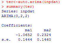
Azure is using the R package auto.arima to do it's forecasting. Auto.arima doesn't look for outliers or level shifts or changes in trend, seasonality, parameters or variance.

Here is the monthly data used. 3.479,3.68,3.832,3.941,3.797,3.586,3.508,3.731,3.915,3.844,3.634,3.549,3.557,3.785,3.782,3.601,3.544,3.556,3.65,3.709,3.682,3.511, 3.429,3.51,3.523,3.525,3.626,3.695,3.711,3.711,3.693,3.571,3.509

It is important to note that when presenting examples many will choose a "good example" so that the results can show off a good product.  This data set is "safe" as it is on the easier side to model/forecast, but we need to delve into the details that distinguish the difference between real "machine learning" vs. fitting approaches.  It's important to note that the data looks like it has been scaled down from a large multiple.  Alternatively, if the data isn't scaled and really is 3 digits out then you also are looking for extreme accuracy in your forecast.  The point I am going to make now is that there is a small difference in the actual forecasts, but the level(lower) that Autobox delivers makes more sense and that it delivers residuals that are more random.  The important term here is "is it robust?" and that is what Box-Jenkins stressed and coined the term "robustness".

Here is the model when running this using auto.arima.  It's not too different than Autobox's except one major item which we will discuss.

. 

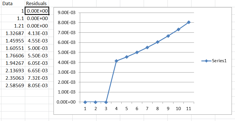
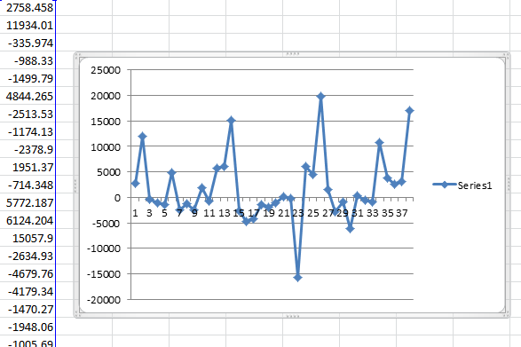
The residuals from the model are not random.  This is a "red flag". They clearly show the first half of the data above 0 and the second half below zero signaling a "level shift" that is missing in the model.

Now, you could argue that there is an outlier R package with some buzz about it called "tsoutliers" that might help.  If you run this using tsoutliers,  a SPURIOUS Temporary Change(TC) up (for a bit and then back to the same level is identified at period #4 and another bad outlier at period #13 (AO). It doesn't identify the level shift down and made 2 bad calls so that is "0 for 3". Periods 22 to 33 are at a new level, which is lower. Small but significant. I wonder if MSFT chose not to test use the tsoutliers package here.

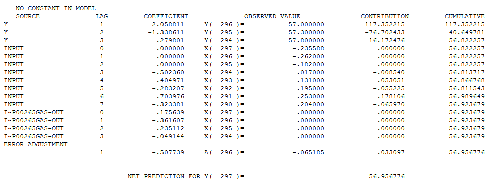
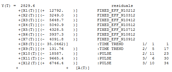
Autobox's model is just about the same, but there is a level shift down beginning at period 11 of a magnitude of .107.

Y(T) =  3.7258                                azure                                                                     
       +[X1(T)][(-  .107)]                              :LEVEL SHIFT       1/ 11    11
      +     [(1-  .864B** 1+  .728B** 2)]**-1  [A(T)]

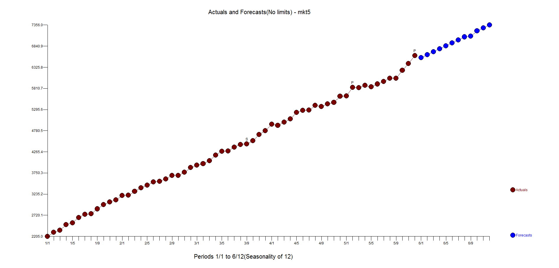
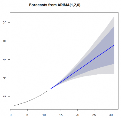
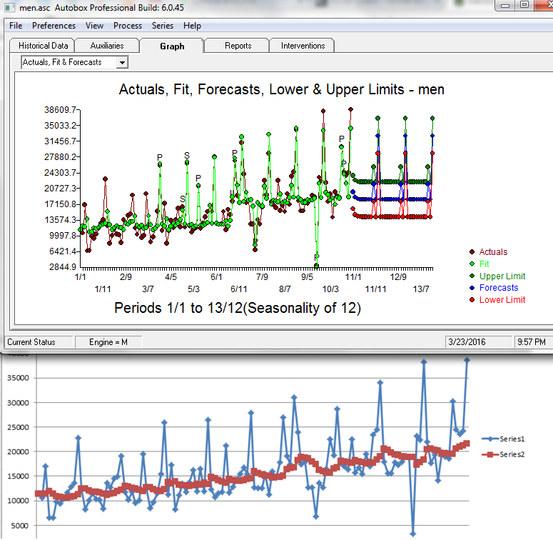
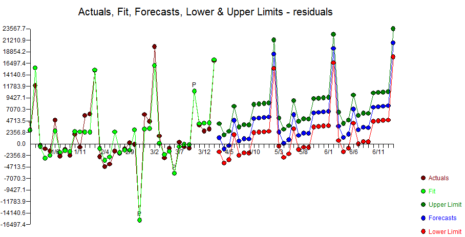
Here are both forecasts.  That gap between green and red is what you pay for.

Note that the Autobox upper confidence limits are much lower in level.

Autobox's residuals are random

IBM released version SPSS Modeler 18 recently and with it a 30 day trial version.

We tested it and have more questions than answers. We would be glad to hear any opinions(as always) differing or adding to ours.

There are 2 sets of time series examples included with the 30 day trial.

We went through the first 5 "broadband" examples that come with the trial that are set to run by default.  The 5 examples have no variability and would be categorized as "easy" to model and forecast with no visible outliers. This makes us wonder why there is no challenging data to stress the system here?

For series 4 and 5 both are find to have seasonality.  The online tutorial section called "Examining the data" talks about how Modeler can find the best seasonal models or nonseasonal models.  They then tell you that it will run faster if you know there is no seasonality.  I think this is just trying to avoid bad answers and under the guise of it being "faster". You shouldn't need to prescreen your data.  The tool should be able to identify seasonality or if there is none to be found.  The ACF/PACF statistics helps algorithms(and people) to help identify seasonality.  On the flipside, a user may think there is no seasonality in there data when there actually is so let's take the humans out of the equation.

The broadband example has the raw data and we will use that as we can benchmark it.  If we pretend that the system is a black box and just focused on the forecast, most would visually say that it looks ok, but what happens if we dig deeper and consider the model that was built? Using simple and easy data avoids the difficult process of admitting you might not able complicated data.

The default is to forecast out 3 periods.  Why? With 60 months of data, why not forecast out at least one cycle(12)?  The default is NOT to search and adjust for outliers.  Why? They certainly have many varieties of offerings with respect to outliers, but makes me wonder if they don't like the results?  If you enable outliers only "additive" and "level shift" are used unless you go ahead a click to enable "innovational", "transient", "seasonal additive", "local trends", and "additive patch". Why are these not part of the typical outlier scheme?

When you execute there is no audit trail of how the model go to its result. Why?

You have the option to click on a button to report "residuals"(they call them noise residuals), but they won't generate in the output table for the broadband example.  We like to take the residuals from other tools and run them in autobox.  If a mean model is found then the signal has been extracted from the noise, but if Autobox finds a pattern then the model was insufficient...given Autobox is correct. :)

There is no ability to report out the original ACF/PACF being reported. This skips the first step for any statistician to see and follow why SPSS would select a seasonal model for example 4 and 5.  Why?

There are no summary statistics showing mean or even number of observations. Most statistical tools provide these so that you can be sure the tool is in fact taking in all of the data correctly.

SPSS logs all 5 time series. You can see here how we don't like the kneejerk movement to use logs.

We don't understand why differencing isn't being used by SPSS here. Let's focus on Market 5. Here is a graph and forecast from Autobox 

Let's assume that logs are necessary(they aren't) and estimate the model using Autobox and auto.arima and both software uses differencing. Why is there no differencing used by SPSS for a non-stationary series? This approach is most unusual. Now, let's walk that back and run Autoboc and NOT use logs and differencing is used with two outliers and a seasonal pulse in the 9th month(and only the 9th month!). So, let's review. SPSS finds seasonality while Autobox & Auto.arima don't.

How did SPSS get there? There is no audit of the model building process. Why?

We don't understand the Y scale on the plots as it has no relationship to the original data or the logged data.

The other time series example is called "catalog forecast". The data is called "men". They skip the "Expert modeler" option and choose "Exponential Smoothing". Why?

This example has some variability and will really show if SPSS can model the data. We aren't going to spend much time with this example. The graph should say it all. Autobox vs SPSS

The ACF/PACF shows a spike at lag 12 which should indicate seasonality. SPSS doesn't identify any seasonality. Autobox also doesn't declare seasonality, but it does identify that October and December's do have seasonality (ie seasonal pulse) so there is some months which are clearly seasonal. Autobox identifies a few outliers and level shift signifying a change in the intercept(ie interpret that as a change in the average).

If we allow the "Expert Modeler", the model identified is a Winter's additive Exponential smoothing model.

We took the SPSS residuals and plotted them. You want random residuals and these are not it. If you mismodel you can actually inject structure and bias into the residuals which are supposed to be random. In this case, the residuals have more seasonality(and two separate trends?) due to the mismodeling then they did with the original data. Autobox found 7 months to be seasonal which is a red flag.

I think we know "why" now.

In 2011, IBM Watson shook our world when it beat Ken Jennings on Jeopardy and "Computer beats Man" was the reality we needed to accept.

IBM's WatsonAnalytics is now avalilabe for a 30 day trial and it did not shake my world when it came to time series analysis.  They have a free trial to download and play with the tool. You just need to create a spreadsheet with a header record with a name and the data below in a column and then upload the data very easily into the web based tool.

It took two example time series for me to wring my hands and say in my head, "Man beats Computer".  Sherlock Holmes said, "It's Elementary my dear Watson".  I can say, "It is not Elementary Watson and requires more than pure number crunching using NN or whatever they have".

The first example is our classic time series 1,9,1,9,1,9,1,5 to see if Watson could identify the change in the pattern and mark it as an outlier(ie inlier) and continue to forecast 1,9,1,9, etc.  It did not.  In fact, it expected a causal variable to be present so I take it that Watson is not able to handle Univariate problems, but if anyone else knows differently please let me know.

The second example was originally presented in the 1970 Box-Jenkin's text book and is a causal problem referred to as "Gas Furnace" and is described in detail in the textbook and also on NIST.GOV's website.  Methane is the X variable and Y is the Carbon Dioxide output.  If you know or now closely examine the model on the NIST website, you will see a complicated relationship where there is a complicated relationship between X and Y that occurs with a delay between the impact of X and the effect on Y (see Yt-1 and Yt-2 and Xt-1 and Xt-2 in the equation).  Note that the R Squared is above 99.4%!  Autobox is able to model this complex relationship uniquely and automatically.  Try it out for yourself here! The GASX problem can be found in the "BOXJ" folder which comes with every installed version of Autobox for Windows.

Watson did not find this relationship and offered a predictive strength of only 27%(see the X on the left hand of the graph) compared to 96.4%.  Not very good. This is why we benchmark. Please try this yourself and let me know if you see something different here.

Autobox's model has lags in Y and lags in the X from 0 to 7 periods and finds an outlier(which can occur even in simulated data out of randomness).  We show you the model output here in a "regression" model format so it can be understood more easily. We will present the Box-Jenkins version down below.

Here is a more parsimonious version of the Autobox model in pure Box-Jenkins notation.  Another twist is that Autobox found that the variance increased at period 185 and used Weighted Least Squares to do the analysis hence you will see the words "General Linear Model" at the top of the report.

You were taught and told through books, teachers, websites and your software that your AR model coefficient can't be outside the -1 to +1 region. This is also often stated as that "unit root" needs to be outside the unit circle, but this just isn't true. A criticism of Box-Jenkins modeling was that it wasn't applicable to growth models.

Ok, but why does that matter to me? Well, it matters to you as that means you have been operating under an assumption that limits your modeling to handle explosive data from perhaps a product launch where sales really take off. Typically, the long run forecasts from such a time series are not usually realistic, but the mid to short are useful.

Let's look at annual data that has explosive and "multiplicative" growth.

1.1 1.21 1.33 1.46 1.61 1.77 1.95 2.14 2.36 2.59   <<<<<----------  Note how the incremental differences keep getting larger(ie .11, .12, .13, .15, .16, .18, .19, .22, .23)

If we modeled this based on what we were taught or using a typical forecasting tool, it would build a model with double differencing and an AR 1. The forecasts The residuals would show that the model didn't actually capture the signal as it was constrained by the bounds of the unit circle(-1 to +1).

ARIMA(1,2,0) Coefficients: ar1 0.6868 s.e. 0.2121 sigma^2 estimated as 0.0001214: log likelihood=27.48 AIC=-50.97 AICc=-48.97 BIC=-50.57

Below are the forecasts.  Note the almost flat forecast and lack of explosive growth.

Most software and people ignore the residual plot.  This is a big mistake.  This is a clear way of checking to see if the model was built in a robust manner by checking if the residuals are random or also known as Normal Independently Identically Distributed (N.I.I.D.) which is the ASSUMPTION that the whole modeling process is built upon, but again ignored.  The residuals are not random at all.

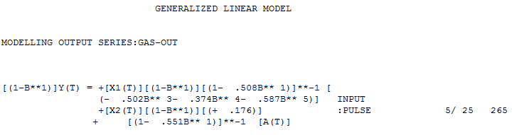
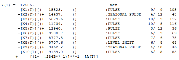
If we ignore the unneeded unit circle constraint,  the model would be again double differencing with an AR1 coefficient that is 1.1 and very much OUTSIDE the unit circle and very estimable!

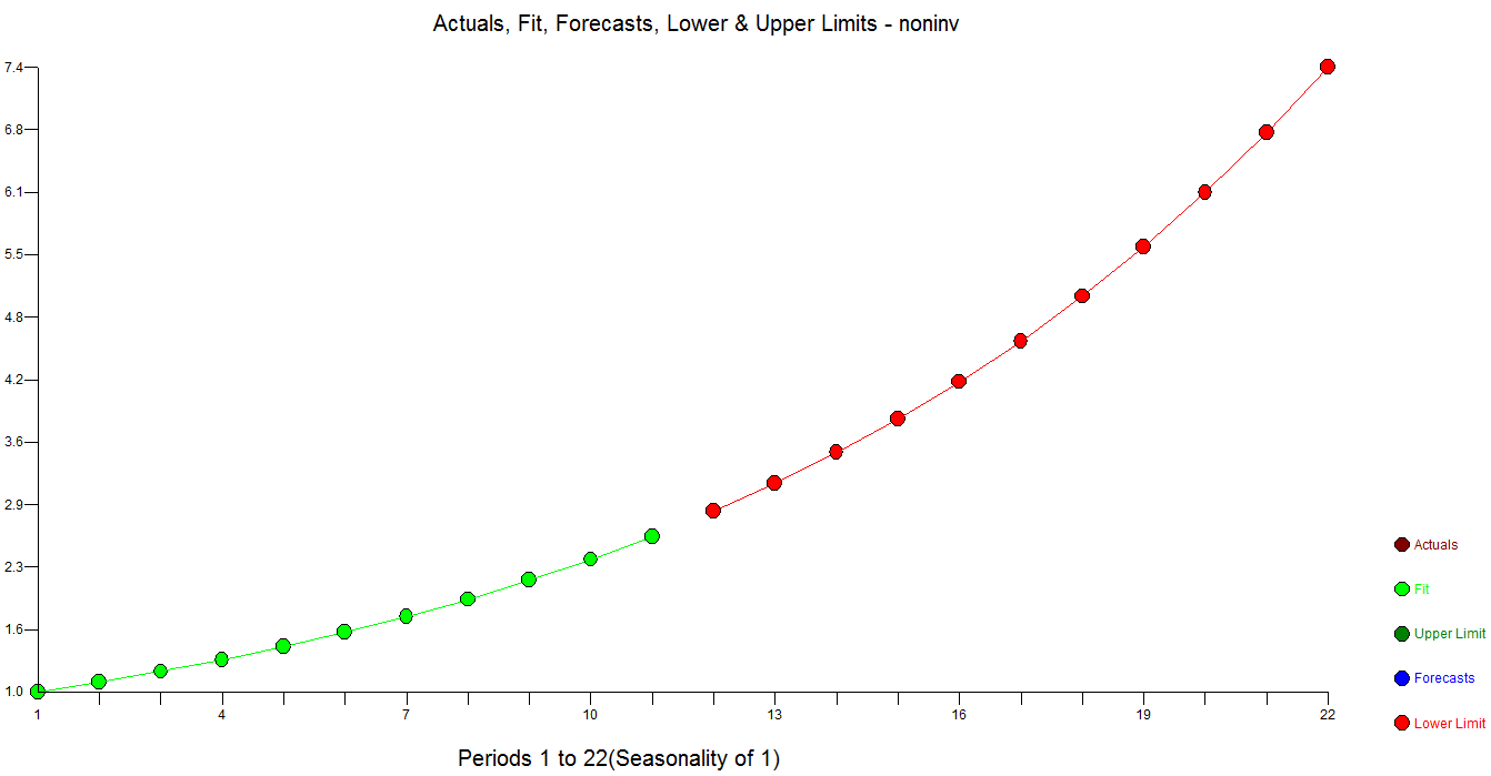
[(1-B**1)][(1-B**1)]Y(T) = .82601E-07 + [(1- 1.1000B** 1)]**-1 [A(T)]