2.6 Effective Forecasting of Slow Movers
2.7 Danger in Least Squares Regression
3.1 Intervention Modeling Limitation
3.2 Number of Data Points Needed
1 Introduction
Demand planning is one of the single biggest challenges of inventory optimization. All decisions made today are based on what we believe will happen tomorrow. The more we know about what will happen, the better one can prepare for such challenges or take advantage of opportunities.
AUTOBOX, based on the ground breaking Box-Jenkins methodology, is an expert system that can be used to model and forecast both univariate and multivariate time series. G.E. Box and G.M. Jenkins developed what is widely regarded to be the most efficient and accurate statistical forecasting technique in 1976. They suggested a broad class of underlying statistical models of demand patterns, as well as a procedure for selecting the appropriate member of the class based on the historical data available. It differs from traditional techniques by not assuming a model from a predefined list of models, but by identifying (and building) the model itself from the data.
The result of the research by Box and Jenkins (now know as the Box-Jenkins method), addresses the need to model both Univariate and Multivariate models:
Univariate Model: Predict future values of a time series solely on the basis of past values of the time series. Box-Jenkins uses ARIMA (auto-regressive integrated moving-average) for modeling such time series.
Multivariate Model: Predict future values not only based on the past values, but also on secondary time series that incorporates demand impacting cause variables.
AUTOBOX is attractive to both the expert and the non-expert. The expert can apply their knowledge to control the flow of modeling and estimation. The non-expert can use it as a “statistician-in-the-box” without having to understand the math behind the AUTOBOX heuristic.
2 Forecasting Strengths
2.1 Tailored Model
The approach is to develop the model identification, estimation and diagnostic feedback loop as originally described by Box and Jenkins.
Box-Jenkins forecasting models are based on statistical concepts and principles and are able to model a wide spectrum of time series behavior. Instead of selecting a model from a user or system-defined set of models, AUTOBOX uses a systematic approach for tailoring the forecast model to each time series.
The aim of AUTOBOX is to deliver simple answers when simple answers are appropriate and complex answers when complex answers are appropriate.
2.1.1 Modeling Procedure
Normally one would list possible models without a clue as to how the models inter-relate. The typical selection process offered by simple software is Exponential Smoothing, X-11, Trend Models, Regression Models and Weighted Averages. Very little, if any is made of the family tree of forecasting and how models relate to each other. Model selection is done on either an out-of-sample basis or some within sample statistic. The out-of-sample approach fails a test of objectivity because it hinges on the number of values that was withheld.
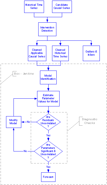
The Box-Jenkins methodology consists of a four-step iterative procedure.
1. Tentative identification: historical data are used to tentatively identify an appropriate Box-Jenkins model.
2. Estimation: historical data are used to estimate the parameters of the tentatively identified model.
3. Diagnostic checking: various diagnostics are used to check the adequacy of the tentatively identified model and, if need be to suggest an improved model, which is then regarded as a new tentatively identified model.
4. Forecasting: once a final model is obtained, it is used to forecast future time series values.
Before tentatively identifying a model, the time series must be converted into a stationary time series if it is not.
Stationary Time Series: The mean and the variance are constant over time.
Non-Stationary Time Series: Either or both the mean and / or the variance change over time.
2.1.2 Model Components
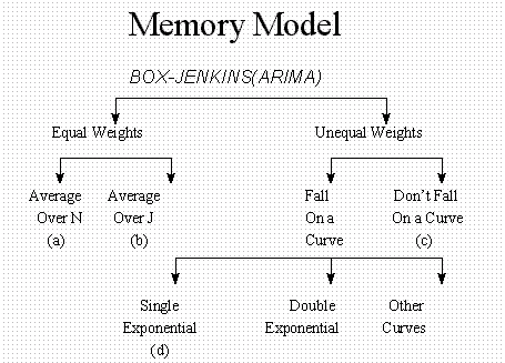
The three components of a Box-Jenkins forecasting model are:
· Dummy variables
· History of the series of interest
· Causal variables i.e. potentially supporting series
The dummy variables are used to identify and store information of pulses, level shifts, outliers, inliers or local time trends.
The final model will satisfy both:
· Necessity tests that guarantee the estimated coefficients are statistically significant.
· Sufficiency tests that guarantee that the error is unpredictable on itself, not predictable from the set of causal data or their lags and has a constant mean of zero.
2.2 Detects Outliers, Inliers, Seasonal Pulse, Level Shifts & Trends
AUTOBOX follows a systematic process to simulate a skilled statistician identifying intervention variables or important pulses. Using a data mining process, AUTOBOX will mechanically search for the least believable hypotheses and test it to determine whether or not such data point/s are to be regarded as outliers, inliers, seasonal pulses, level shifts or local time trends.
2.2.1 Outliers
If the outlier is outside of a particular probability limit (95% or 99%), one will first formulate a hypothesis and try to reject it. If not, the pulse is regarded as an outlier and will be removed from the observation. This deletion or adjustment of the value so that there is no outlier effect is equivalent to augmenting the model with a 0/1 variable (dummy) where a 1 is used to denote the time point and 0's elsewhere.
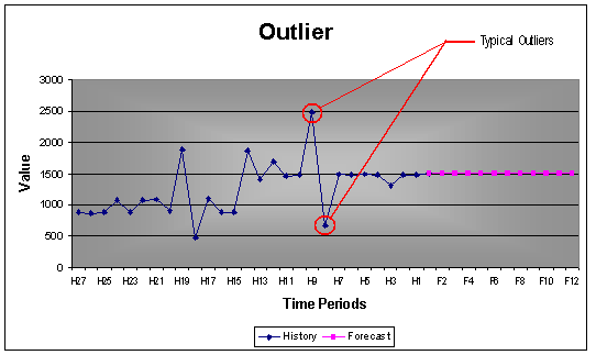
Example: 27 monthly values with a seasonality of 12. The forecast clearly shows that the outliers were not used for the forecast.
2.2.2 Inliers
The effect of inliers is just as serious as outliers. Inliers are too normal or too close to the mean. If ignored inliers will bias the identification of the model and its parameters.
To evaluate each and every unusual value separately is inefficient and misses the point of intervention detection or data scrubbing. A sequence of values may individually be within "bounds", but collectively might represent a level shift that may or may not be permanent. A sequence of "unusual" values may arise at a fixed interval representing the need for a seasonal pulse "scrubbing”. Individual values may be within bounds, but collectively they may be indicative of non-randomness. To complicate things a little bit more, there may be a local trend in the values.
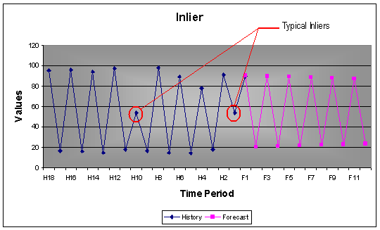
Example: 18 monthly values with a seasonality of 12. The two inliers were removed from the data used to develop the model.
2.2.3 Seasonal Pulses
Seasonal pulses are repetitive pulses over time. It can be for a short period of time, for example holiday or over a longer period such as ski equipment in Aspen during winter.
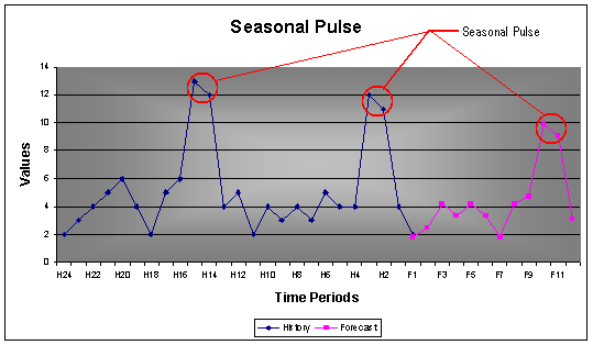
Example: 24 monthly values with a seasonality of 12. The seasonal pulses over periods H2 – H2 and H14 – H15 were forecasted by AUTOBOX over period F10 – F11.
2.2.4 Local Time Trends
Local time trends in time series require identification of the break points and then estimation of the local trend. It often happens that a time series appears to have a trend, but is not. If the trend is not convincing, AUTOBOX will not apply a trend to the forecast.
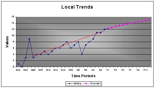
Example-1: A time series with 24 monthly values with a seasonality of 12 with trend.
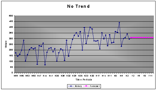
Example-2: 59 monthly values with a seasonality of 1, since it is yearly values. AUTOBOX does recognize the level shift, but does not forecast a trend, since the signal for a trend is not convincing.
2.2.5 Level Shifts
Being able to identify level shifts are important when forecasting. It often happens that an item makes a clear shift due to demand circumstances that changes, if the forecast tool does not recognize the shift, the forecasts will be diluted with values that are not applicable anymore.
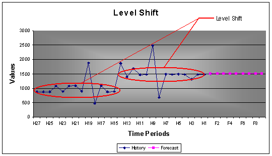
Example: 24 monthly values with a seasonality of 12. The AUTOBOX forecast is clearly based on only the last 14 periods.
2.3 Flexible yet Robust
There is complete control over the statistical sensitivities for the inclusion/exclusion of model parameters and structures. These features allow the user complete control over the modeling process. The user can let AUTOBOX do as much or as little of the model building process as the user or the complexity of the problem dictates. At the same time, AUTOBOX eliminates unnecessary structure such as statistically unimportant cause variables.
2.3.1 Artificially Increasing Sample Size
The number of degrees of freedom for the significance test is falsely increased when one uses 240 hourly data points instead of 4 monthly observations. The sample size is not really increased, although statistical calculations are done as if it was. By taking observations at closer intervals we create a time series with higher and higher autocorrelation.
AUTOBOX with the use of filtering and pre-whitening will remove such autocorrelation.
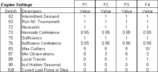
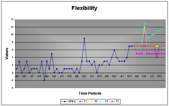
2.3.2 Flexibility
Having a flexible tool where a knowledgeable person can guide AUTOBOX is important, especially for more important / valuable forecasts that are reviewed after creating the automatic forecast. If a company are making 80% of there revenues on a handful of items, they will definitely do there best ensuring that nothing goes wrong with these items.
AUTOBOX is controlled by 155 switches that can be used to increase the accuracy of the forecast. Less experienced users can use some switches, while other switches are recommended to be used only by advanced users. The best approach is to let the default engine take care of all forecasts and only review the most important forecast that are crucial to the company.
2.3.3 Spurious Correlation & Causal Variables
Spurious relation or correlation is a situation in which measures of two or more variables are statistically related, but are not in fact causally linked. This is usually because the statistical relation is caused by a third variable. When the effects of the third variable are taken into account, the relationship between the first and second variable disappears.
An analyst who takes correlation results as indicating a causal relationship makes the same mistake as a person drawing conclusions such as "fireman cause damage because the more fireman you have at a fire the more damage is reported”.
This apparent cross-correlation is based on the (incorrect) assumption that the series have no internal autocorrelation. Once you account for the time series or auto-projective component the cross-correlation becomes non-significant. The concept of incorporating needed, but omitted variables is clear in time series because the concomitant variable is usually obvious after its presence has been detected via ARIMA structure with a conclusion that the X variable is not significant above and beyond the historical impact of Y. There are many cases where the ARIMA structure reduces the error variance, enables a clearer picture and the significance of a candidate variable.
In a similar vein, it was reported that in a certain African country epidemics were high were there was relatively a higher proportion of doctors. We might as well attribute the epidemics to the presence of the doctors!! These kinds of stories have been used to demean the practice of statistics; rather it demeans the incorrect utilization of cross-sectional statistical tools on time series problems. Statistics is not at fault it is the unwary practitioner and/or inefficient statistical tools.
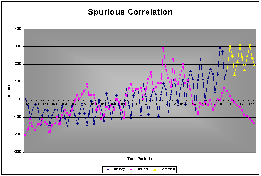
Example: Here is an example of two economic variables that does have a cross-correlation, but when studied with AUTOBOX the predictor variable is not proven to have any information. It is evident that the forecast is not influenced by the prediction of the causal.
2.4 Automated Modeling
AUTOBOX offers a total automation of the modeling and forecasting tasks, therefore, it can be recommended to practitioners who must process large amounts of data automatically. Even though this automated process is somewhat slower than the very simple models (like the more simplistic moving average algorithms), it allows for a set of robust forecasting programs to forecast hundreds of thousands or even millions of items.
2.4.1 Automatic Model Identification
AUTOBOX uses a set of dummy variables when searching for patterns that should be included in the model. This is part of the automatic model identification that does not need any user interaction. If the signal is strong a trend can be identified with only a few data points.
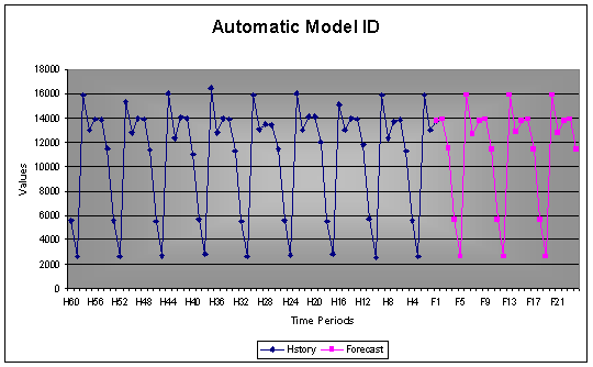
Example: This example shows how AUTOBOX forecasted a repeating pattern by using automatic model identification.
2.5 Causal Variables
It has the additional benefit of optimally incorporating variables that cause changes to demand patterns. We know that the past never "causes" the future. The future is "caused" by marketing decisions, competitor action, holiday effects, etc. Optimally combining information in these variables as well as the past sales (or more correctly past demand) history, can be hugely effective.
Causal variables of both deterministic and stochastic nature can be applied. This means that the impact of such a causal can be restricted to a specific time period (deterministic) or it can have lead or lag effects (stochastic).
2.5.1 Determining the Effect of a Causal
The first step for AUTOBOX is to determine whether or not the causal is applicable to the time series to be forecasted. Secondly the magnitude of the effect needs to be estimated. The outliers and inliers are removed before proceeding with the forecast. Otherwise the magnitude of the effect may be deluded.
Example: This example demonstrates how outliers are excluded from the determining the magnitude of the causal effect. If all 5 causal variables were included the causal pulse should be 10. Since the one causal is identified as an outlier, the magnitude is correctly calculated to be 12.
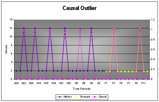
The simplified calculation:
[Sum of quantities at Causal Variables] / [Number of Causal Variables] = [60] / [6-1]
= 12
2.5.2 Deterministic Causal
If a causal variable will only effect that specific period wherein the causal occur, one need to use a deterministic causal. The trading days per month only effects the sales of this month, it does not influence the sales of the previous or the month thereafter. Another example is effect of weather on ice-cream sales. These are typical examples of causal variables that only effect the period of occurrence.
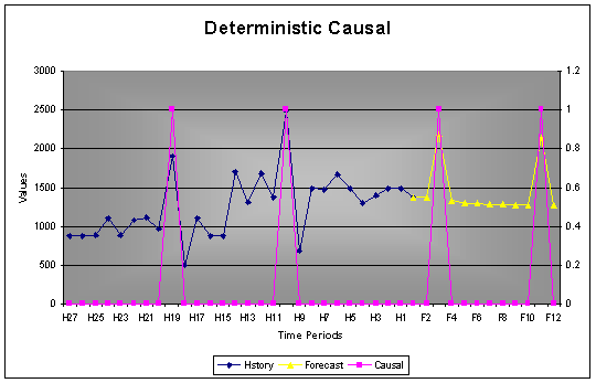
Example: Although it seams that there is a lagging effect in the data, by choosing a deterministic causal, one confirms that the causal has nothing to do with the reduction on sales after the peak. AUTOBOX will not include the reduction except if it is recognized as a seasonal trend equally spread over time.
2.5.3 Stochastic Causal with Lag Effect
It often happens that a causal, such as a promotion, does have a lag effect. AUTOBOX will include such signal when using a stochastic causal.
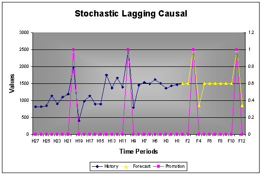
Example: Using the same time series as for the deterministic example just with a stochastic type of causal instead of deterministic, shows how AUTOBOX does pick up the drop after the causal variable (probably promotions).
2.5.4 Stochastic Causal with Lead Effect
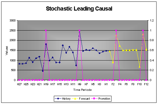
Causal variables can also have a lead effect. In the case where a price cut is expected beforehand or one is expecting an upgraded version of a product to be launched soon, one may hold back before buying. This is a typical lead situation that is well catered for when using AUTOBOX.
2.6 Effective Forecasting of Slow Movers
Many companies are faced with the difficulty of forecasting slow moving items with sparse data. This sequence can't be treated as an ordinary uninterrupted time series because of the non-constant time differential. Additionally the treatment of small integers as if they were continuous, stretches one of the assumptions underlying continuous distribution modeling.
AUTOBOX introduces a method that forecasts the quantity and the intervals between sales separately. This way the many zeros do not delude the actual quantities and inelegance is added to forecasting when the next sale may occur.
By default all items where more than 50% (which can be adjusted) of the data point are zero will be modeled using Intermittent Demand.
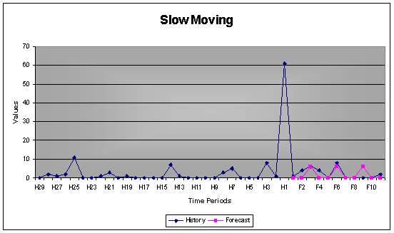
Example: Showing the AUTOBOX intermittent demand forecast compared with the actual data for the time series.
2.7 Danger in Least Squares Regression
The robustness of AUTOBOX is again proven with the following example.
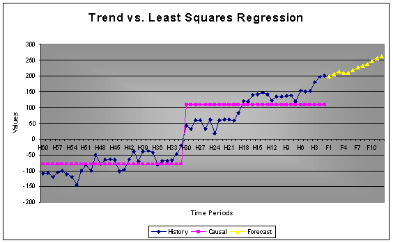
Example: In this example a causal was added to a time series, using standard least squares regression concludes that the cause variable is statistically significant. The reason for the significance is that the mean for the first 30 observations is statistically significantly different from the mean of the last 30 observations. In this case, as identified by AUTOBOX, one should not be concerned with a test of the hypothesis of 2 means, because the series has trend.
3 Forecasting Weaknesses
3.1 Intervention Modeling Limitation
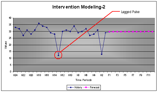
The purpose of intervention modeling is to identify pulses that may either be of importance or just an outlier. AUTOBOX does not pickup single pulses if any of the points are lagging or leading. To ensure that such single pulses are included in the model, one must add a causal series to support the qualitative information behind including such single pulses.
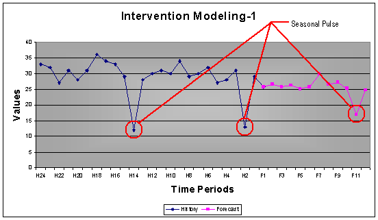
Example: The first graph shows where intervention modeling identified the low at H11 & H23 as seasonal and forecasted accordingly. The second graph shows the weakness where the lagged low at H12 was not linked to the low at H23.
3.2 Number of Data Points Needed
A rule of thumb is to have 3 times the seasonal period’s data for the Box-Jenkins methodology. Assuming a seasonality of 12 then preferably one requires 36 data points. The less data points the more difficult it will be to identify a signal or pattern. The more noise there is within the time series the more data will be required to separate noise from signal.
AUTOBOX, however, addresses this issue, using a candidate model to estimate and revise based upon the information in the residuals. This allows AUTOBOX to forecast patterns with less data than normally required.
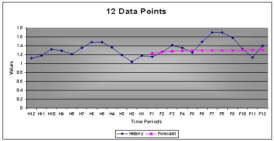
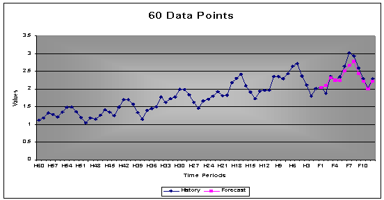
Example: The first graph shows the forecast with only 12 data points. As shown, the forecast is based on the mean, since no signals could be identified. The same time series is shown in the second graph. This time 60 data points were used instead of 12. With more data the accuracy improved from 89% to 95%. The second graph includes patterns that could be identified with more data. Note that the first forecast on 12 data points were still a good forecast, the second one was just better as one would have expected with 4 times more data.
3.3 Modeling Time
Due to the massive computation required to automate the Box-Jenkins methodology, and the technology used by AUTOBOX, the forecast engine is significantly slower than the standard Ability – Inventory Optimization forecast engine computing a best fit on conventional forecasting methods. This concern is partly overcome by scheduling forecast jobs. The Scheduler can use the server processors as well as PCs’ made available via the LAN, which can be used when they are idle.
It is important to remember that using causal variables does increase computation time. For the sake of time, it is recommended not to assign default causal series to all items, but rather to assign causal series to items or groups of items where believed to be applicable.
4 Modeling Overview
The forecasting engine is built on the central modeling steps of the Box-Jenkins paradigm. This core is extended by several useful modules such as intervention detection, a simulation option and a few other functions, all of which assist in forecasting.
The flowchart below is a high level overview of the modeling and forecasting approach used by AUTOBOX.
