www.autobox.com - Automatic Forecasting Systems

Tom Reilly
Waging a war against how to model time series vs fitting
A closer look at SAP PAL - If you're not looking for inliers, then you can't see them. You need Autobox glasses to do that!

- Font size: Larger Smaller
- Hits: 39094
- 0 Comments
- Subscribe to this entry
- Bookmark
SAP HANA is a Database. PAL is SAP's modeling tool. SAP's naming conventions are a bit confusing. SAP HANA has a very comprehensive user's guide that not only shows an example model of their "Auto Seasonal ARIMA" model on page 349, but also includes the data which allows us to benchmark against. The bottom line is that the ARIMA model shown is highly overparameterized, ignores outliers, changes in level and a change in the seasonality.
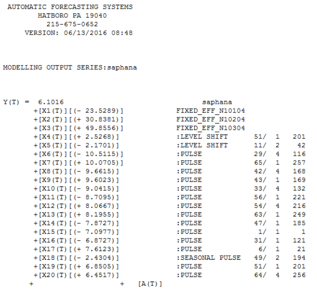
Here is the model built by HANA that we took and estimated in Autobox which matches what SAP shows in their User's guide. We suppressed the identification of outliers, etc. in order to match. None were searched for and identified by SAP. Maybe they don't do this for time series?? We can't tell, but they didn't present any so we can assume they didn't. That's a lot of seasonal factors. Count them....1,2,3,4. That's a red flag of a system that is struggling to model the data. We have never seen two MA4's in a model built by Autobox.

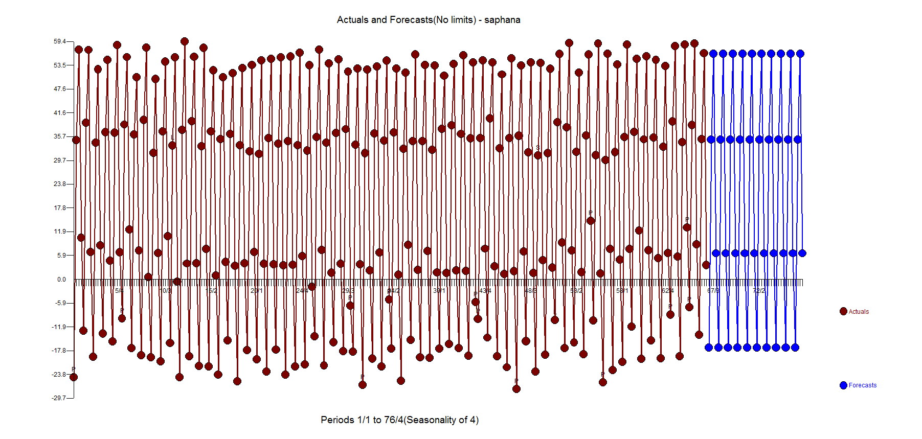
With that said, the truth is the forecast from Autobox and SAP HANA is about identical when using all 264 observations. However, you need to consider other origins. If you go back 7 periods and use 257 observations (and assume the same model which I feel safe doing for this example) to where there were back to back outliers the forecast isn't good. The forecast(as expected) using 256,258,259,260 observations is also bad so yes you want to adjust for outliers and there are consequences if you don't. To reproduce all of this in Autobox, run with Option "4" with this Autobox file, model file and rules.
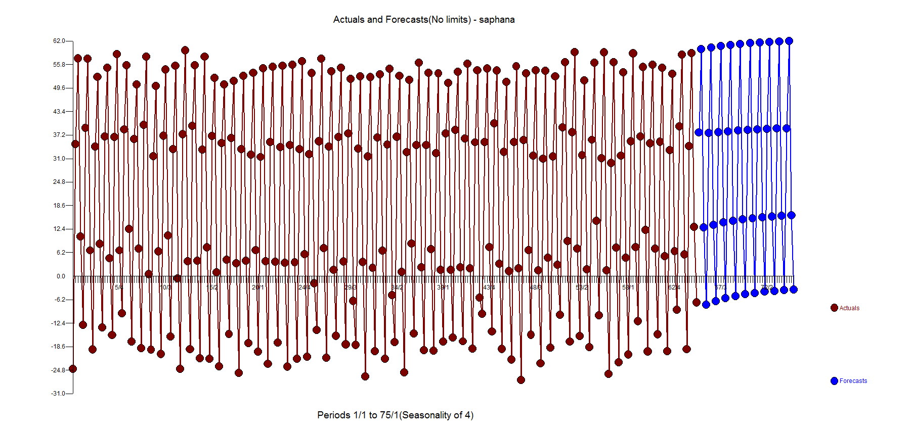
Here is the forecast using Autobox using all the data(SAP HANA is just about the same)
The example is quarterly data for 264 periods. What SAP HANA doesn't recognize(likely others too?) is that with large samples the standard error is biased to providing false positives to suggest adding variables to the model. When this occurs, you have "injected structure" into the process and created a Type 2 error where you have falsely concluded significance when there was none.
The example is a fun one in a couple of ways. The first observation is an outlier. We had seen other tools forecast CHANGE adversely when you deliberately change the first value to an outlier.
The SAP model shown on page 354 uses an intercept AR1, seasonal differencing, and AR4 and two MA4's. Yes, two MA4's.
Let's take a look at what Autobox does with the example.
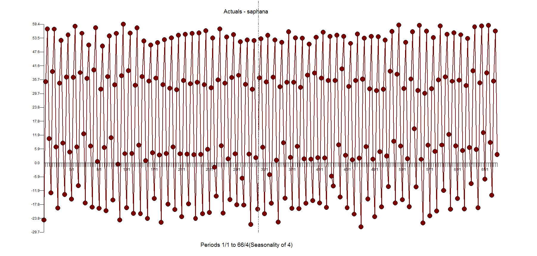
When you look at the plot of the data you, you might notice that the level of the data starts high, goes lower and then goes back to the initial level. this called a "level shift". You can calculate local averages of these 3 groups to verify on your own. of the The biggest culprit is the 4th quarter which seems and then look at the Autobox actual and fit, it becomes easier to see how the data drops down in the middle and then goes back to the previous level.
Autobox uses 3 fixed dummies to model the seasonality. It identifies a drop in volume at period 42 of about 2.17 and then back up to a similar level at period 201. 15 outliers were identified(a really great example showing a bunch of inliers...these won't get caught by other tools - look at periods 21,116,132,168,169,216,250,256,258). A change in the seasonal behavior of period 2 was identified at 194 to go lower by 2.43. An interesting point is that while the volume increased at period 201 the second quarter doesn't.
Here is a plot of the actual and outliers adjusted for just the last 52 observations. This clearly shows the impacts of adjusting for the outliers.
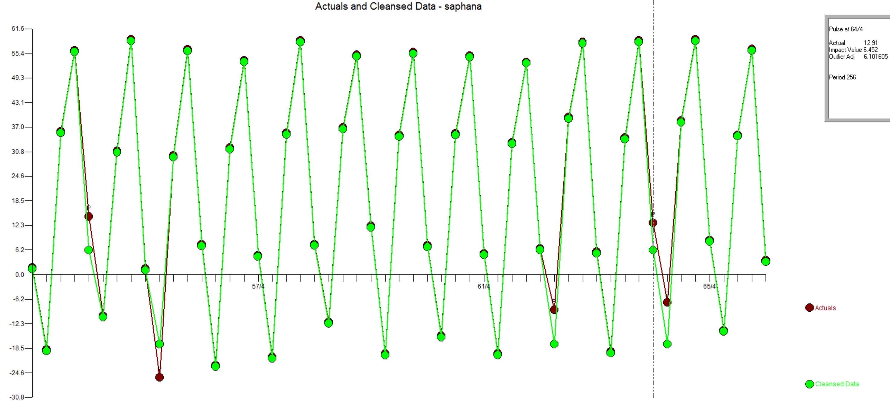
Let's look at the actual and fit and you will see that there are some outliers(not inliers) too(1st observation for example).

Based on the calculated standard error, if you look at the residuals of the Autobox model you will see that lag 1 says it is significant. What we have found out, over the years, is that with large sample sizes this statistical test is flawed and we don't entertain low correlated (.18 for example here) spikes and include them if they are much stronger.
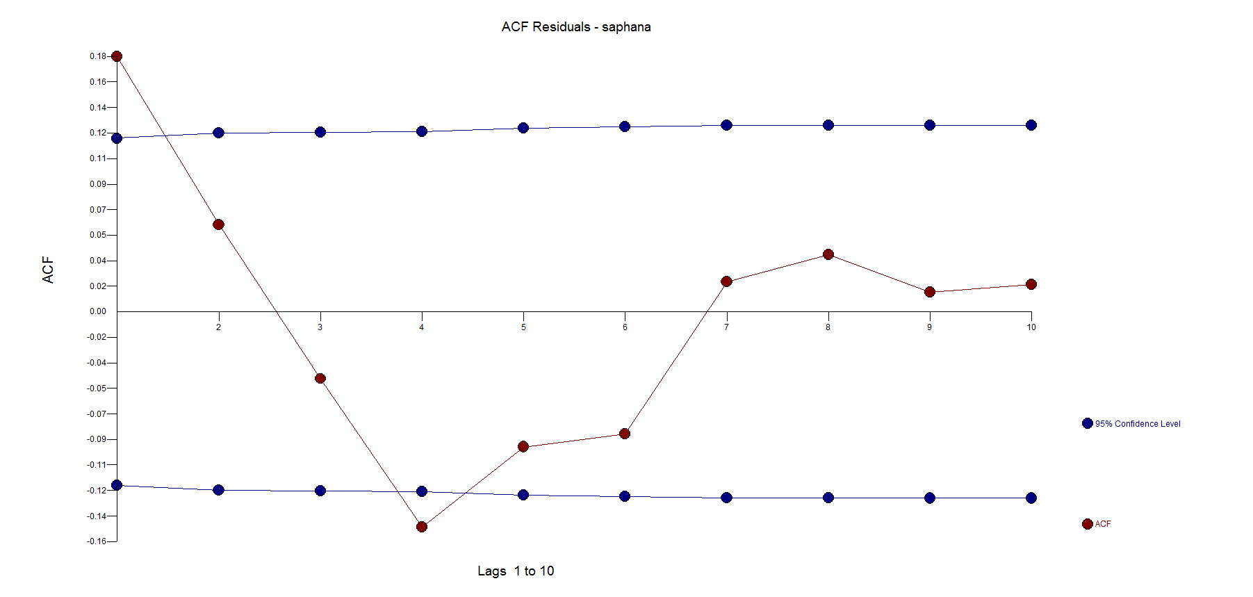
Here are the Autobox random, free of pattern and trend residuals(ie N.I.I.D.):

Comments
-
Please login first in order for you to submit comments