QUESTION:
Most of your competitors
market products that do outlier detection and some sort of adjustment. What is
the big deal with
AUTOBOX in this regard ?
ANSWER:
The answer to this
question hinges on how we compute the standard deviation
for the purposes of determining statistical
significance. Consider
that the standard deviation of the series could be used to normalize the series
to a 0,1
distribution. The
standard deviation as computed by our competitors is based upon the sum of
squares of the values
around the MEAN. The
formula requires that one compute the sum of squares around the EXPECTED VALUE.
The
MEAN is the expected
value if an d only if the series is UNCORRELATED or independent of previous
values. AUTOBOX
correctly computes the
standard deviation, thus correctly assesses unusual values. Consider the
series 1,9,1,9,1,9,9,9,1,9 . The usual, and in this case incorrect ,
computation of the standard deviation would cause a
failure to detect the
anomaly. Replacing the MEAN with the EXPECTED VALUE [Y(t-2)] would result in a
standard
deviation that is
smaller ( a lot smaller ! ) and thus the anomaly in the 7t h value would be
immediately identified.
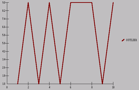
Consider a graphical
presentation of the OUTLIER series 1,1,9,1,9,9,9,1,9
and reflect on the visually obvious !

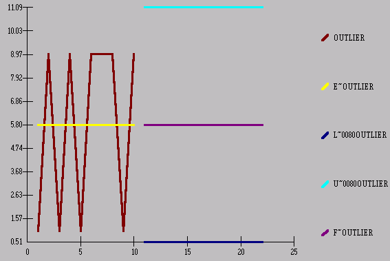
Now, if we were to
compute the standard deviation (4.13) in the traditional way
we would get the
following 80% Confidence Limits

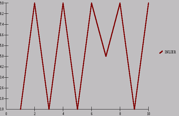
Consider another
example. This time of an INLIER. 1,9,1,9,1,9,5,9,1,9
and reflect on the visually obvious !

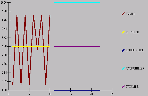
Now, if we were to
compute the standard deviation (3.97) in the traditional way we would get the
following
80% Confidence Limits

The problem or
opportunity in both of these cases is to consider the impact of autocorrelated
data on basic
statistical calculations
and their impact or mostly their lack of impact in adequately describing
statistical
processes. Another way
to consider the effect of autocorrelation is to consider the idea that the RANGE
(max value - min value )
is expected to be approximately 6 times the standard deviation. This is only
true for
Gaussian series with
independent values. The t rue relationship of the RANGEand
the STANDARD DEVIATION
depends on the
autocorrelative structure in the series. The implications are clear ! The idea
that one can mark off
plus or minus k sigma
around the mean and use it as a device to talk about confidence intervals or
limits assumes
independence. If one has
time series data then on average one has autocorrelated data, thus the simple
computation
may be unwise and our no
tion of the range might have to be rearranged.
A RELATED QUESTION:
I want to average the
1-second output of a satellite positioning system for 24 hours (86,400 data
points). This gives a
good estimate of the
true position. The question is, how accurate is the resulting average?
Recalling my statistics
class, I computed the
standard deviation of the 86,400 points and divided it by sqrt(86,400) to get
the standard error
of the mean position.
The resulting value is far too optimistic, I think. The measurement errors are
partly Gaussian
and partly due to a
number of biases that change slowly over a period of minutes. So obviously
there are not 86,400
independent
measurements. Question 1: How does one characterize the variance of data with
such slowly changing
random biases? Question
2: What is the accuracy to be expected from averaging such data over a
specified length of
ANSWER: As you logically concluded your estimated standard
deviation is overly optimistic. This is due to the fact
that you do not have independent samples.
The 86,400 values represent a set of autocorrelated values and thus we must
discuss time series analysis. I would think that an ARIMA
model suitably extended to include pulses, level shifts,
seasonal pulses and local time trends might paint a more
realistic picture. Care must be taken to insure that the
variance of the errors is constant or at least not proven
to be different and furthermore that the estimated parameters
are invariant over time. Given these conditions one might
be able to estimate the standard deviation of the constant in
the appropriate Transfer Function model. The heart of the
matter is that the standard deviation is defined with respect
to the EXPECTED VALUE not necessarily the mean.
