Standard Deviation, Variance, Means and Expected Values The data values in a sample are usually not all the same. Note that if all the sample values are the same the variance is null. This variation between values is called dispersion. The variance of a random variable is a positive number describing how likely the spread of the values of the random variable are predicted; the smaller the variance, the tighter the spread or dispersion around the mean. The variance measures how closely concentrated values are around the expected value of the distribution is; it is a measure of the 'spread' of a distribution about its average value (sic).

where E(X) is the expected value of the random variable X. NOTE: that the formula uses the expected value not the mean. The mean is equal to the expected value only when the values are independent of each other.

As a reflection, one can note that the the Expected Value can always be thought of as some kind of average , not necessarily an equally weighted average.

Some examples of E(X) are:

If the model is X(T) = Constant + a(t) then the E(X) = Constant

If the model is X(T) = Constant + .7 X(t-1) + a(t) then the E(X) = Constant/[1 - .7]

If the model is X(T) = X(T-2) + a(t) then the E(X) = X(T-2)

Sample variance is a measure of the spread of or dispersion within a set of sample data.

IF we assume that the expected value is equal to the mean then what follows is true: The sample variance is the sum of the squared deviations from their average divided by one less than the number of observations in the data set. For example, for n observations x1, x2, x3,....., xn with sample mean:
the sample variance is:

We compute the standard deviation by taking the square root of the variance:

The assumption of independence of observations implies that the most recent data point contains no more information or value than any other data point, including the first one that was measured. In practice, this means that the most recent reading has no special effect on estimating the next reading or measurement. In summary, it provides no information about the next reading. If this assumption (i.e. independence of all readings) holds, this implies that the overall mean or average is the best estimate of future values. If, however, there is some serial or autoprojective (autocorrelation) structure the best estimate of the next reading will depend on the recently observed values. The exact form of this prediction is based on the observed correlation structure. Stock market prices are an example of an autocorrelated data set. Weather patterns move slowly, thus daily temperatures have been found to be reasonably described by an AR(2) model which implies that your temperature is a weighted average of the last two days temperature. Try it and see if doesn't work !

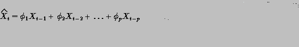
We compute the Expected Value by the following weighted average (Note that if we have a p equal to the actual number of vales recorded (n) AND all weights equal to 1/p then we have a formula for the mean):

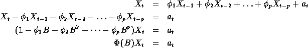
In general terms the Expected Value or Weighted Average is:

and since the Expected Value of the error term is zero, we get:

For example the model might be as simple as:

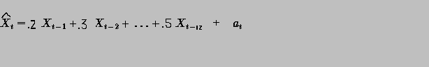
and since the Expected Value of the error term is zero, we get:

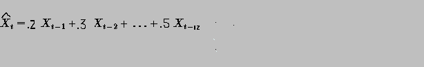
In our example here the model is simply a lag2 autoregressive:

The variance is then computed as the sum of squares around the Expected Value and not the simple average:

The standard deviation follows as usual:

CLICK HERE:Home Page For AUTOBOX