Regression models versus transfer function models

A very natural question arises in the selection and utilization of models.

One asks, "Why not use simple models that provide uncomplicated

solutions?" The answer is very straightforward, "Use enough complexity

to deal with the problem and not an ounce more". Restated, let the

data speak and validate all assumptions underlying the model. Don't

assume a simple model will adequately describe the data. Use

identification/validation schemes to identify the model.

Since regression is a particular subset of a transfer function, it

is possible to constrain the transfer function to deliver regression

results. The following is a development of a transfer function model

from the bottom up. In other words, we will start with a simple model

and allow complications to enter one-by-one. In this manner, we will

show what the real requirements are for a simple regression model.

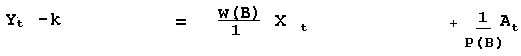
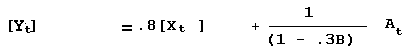
simple model:

where Y_t = Endogenous (output); B0 = constant; B1 = coefficient for X_t;

X_t = Exogenous (regressor); A_t = error term

Restating in terms of a more general class, we get:

Where B0 = k; B1 = W0

Introducing the notion of a polynomial, we get:

W(B) = W0; and in general B^k X_t = X_t-k

or specifically (1 period lag) B¹ X_t = X_t-1 or (no lag) B⁰ X_t = X_t

 Also note that B^k X_t = X_t-k

Incorporating the multiplicative identity element (1) doesn't change anything.

Recognizing that there might be the need for an autoregressive

process to compensate for omitted X's we get the following:

P(B) = 1 for the null case

Recognizing that there might be the need for a moving average

process to compensate for omitted X's we get the following:

P (B) = 1 ; T(B) = 1 for the null case

In general P(B) = 1 - P₁B¹  - P₂B² - P₃B³ - P₄B⁴ + ……. - P_pB^p

T(B) = 1 - T₁B¹  - T₂B² - T₃B³ - T₄B⁴ + ……. - T_qB^q

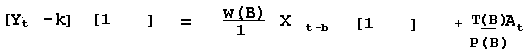
Recognizing that there might be the need to incorporate a period

of delay (b) before Y responds X we get:

If there is no delay then b=0; b= delay or "dead time" before Y responds to X.

Incorporating the identity element (1) doesn't change anything.

Recognizing the possibility that the level of Y might depend on

changes in X, rather than the level of X suggests:

P(B) = 1 ; T(B) = 1 {[1-B^o]}^d = 1 for o =0 & d =0

More generally to reflect the particular series (X).

 w(B) = w0 where B¹ X_t = X_t-1 and in general B^k X_t = X_t-k

b= delay or "dead time"

P(B) = 1 ; T(B) = 1 {[1-B^o1]}^d1 = 1 for o1 =0 & d1 =0

Recognizing the possibility that changes in Y might depend on

changes in X, leads to:

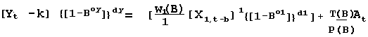
{[1-B^oy]}^dy = 1 for oy =0 & dy =0

Recognizing the possibility that changes in X effect a sequence of Y's leads to a dynamic

model of: 

w(B) = w0 where B¹ X_t = X_t-1 and in general B^k X_t = X_t-k

b= delay or "dead time"

P(B) = 1 ; T(B)=1; D(B)=1 {[1-B^o1]}^d1 = 1 for o1 =0 & d1 =0

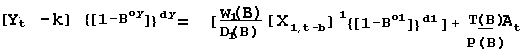
  {[1-B^oy]}^dy = 1 for oy =0 & dy =0; W(B)/D(B)=W'(B)

 Note that W(B)/D(B) can be non-parsimoniously restated W'(B). We prefer W(B) and D(B) in order to minimize the number of coefficients.

Incorporating the identity element (1) for an appropriate power

transformation to de-couple linear dependence between the first and

second moment delivers:

w(B) = w0 where B¹ X_t = X_t-1 and in general B^k X_t = X_t-k

b= delay or "dead time"

P(B) = 1 ; T(B)=1; D(B)=1 {[1-B^o1]}^d1 = 1 for o1 =0 & d1 =0

  {[1-B^oy]}^dy = 1 for oy =0 & dy =0

Allowing these power transforms (^ay , ^a1) to be other than unity leads to:

w(B) = w0 where B¹ X_t = X_t-1 and in general B^k X_t = X_t-k

b= delay or "dead time"

P(B) = 1 ; T(B)=1; D(B)=1 {[1-B^ox]}^dx = 1 for o1 =0 & d1 =0

a is the power transformation ranging from:

-1 inverse

.5 inverse square root

0 logarithm

.5 square root

1 none

For n regressor series we get:

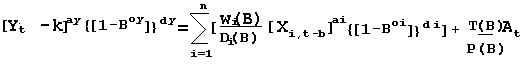
w(B) = w0 where B¹ X_t = X_t-1 and in general B^k X_t = X_t-k

b= delay or "dead time"

Thus the ordinary regression model is seen to be a particular

subset of a more powerful class of model where the following set of

assumptions are in place: 

. power transforms are known or assumed for all series

. the delay is known b = 0

. the required level of differences is known for all series

. the form of the distributed lag structure W(B) is known for all series

. the form of the dynamic lag structure D(B) is known for all series

. the AR lag structure P(B) is known

. the MA lag structure T(B) is known

These are the restrictions that shackle the transfer function when

you assume the ordinary regression model. Thus the model is:

SIDEBAR ON KOYCK:

Another ad-hoc model is popularly known as "polynomial distributed

lags".

w(B) = a polynomial of order L, whose coefficients can be described

by a polynomial of the order L.

E.G. A QUADRATIC

LET W_i = a_o + a_i i + a₂ i²

In the Koyck method, these coefficients are assumed to exponentially decay.

 NUMERICAL EXAMPLE

Sometimes an example can clear up algebraic confusion.

generalizing

generalizing to include seasonal differencing of order 12 for Y

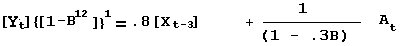
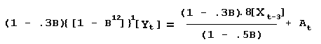
generalizing with a dynamic component; D(B) = 1 - .5B

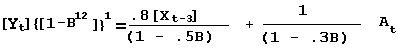
We will revert to no log transformation for simplicity sake. Multiplying through by 1-.3B to clear fractions:

 and in a rearranged or expanded form:

 Since (1- .3B)(1 - B¹² ) = 1 - .3B - B¹² + .3B¹³

We get:

  (1-.3B-B¹²+.3B¹³) Y_t = (.8)[ (1 - .3B][1 + .5B + .25B² + .125B³)] X_t-3 + A_t

(1-.3B-B¹²+.3B¹³) Y_t   = (.8)[ (1 + 2B¹ + 1B² + .5B³ + .25B⁴ + .125B⁵ + .0625B⁶ +…… ] X_t-3 + A_t

(1-.3B-B¹²+.3B¹³) Y_t   = [.8B⁰ + 1.6 B¹ + .8B² + .4B³ + .2B⁴ + .1B⁵ + .05B⁶ +…… ] X_t-3 + A_t

Truncating at lag 9 we get:

(1-.3B-B¹²+.3B¹³) Y_t = + .8X_t-3 + 1.6X_t-4 + .8X_t-5 + .4X_t-6 + .2X_t-7 + .1BX_t-8 + .05X_t-9 + A_t

leading to:

Y_t = .3Y_t-1 +Y_t-12 - .3Y_t-13 + .8 X_t-3 + 1.6 X_t-4 + .8 X_t-5 +.4 X_t-6 + .2 X_t-7 + .1BX_t-8 + .05X_t-9 + A_t

This model that we have built might look like a typical regression model. It does, but the fact remains that we took a much different course…we proceeded through the identification of the model form and arrived with this model. A typical approach might be to start with this model and run it in EVIEWS and whatever variables that aren't significant are removed and presto we have our answer. It should also be noted that the number of coefficients are more than what was really necessary when viewed as a tran sfer function model. This is called overparameterization. When this model is estimated using typical regression the coefficients will be different than the DERIVED coefficients as shown above.

The above equation can be generalized to have >1 endogenous (dependent) variables. This particular problem is referred to as VECTOR ARIMA (VARIMA) where M endogenous variables must be predicted using J exogenous variables. The difference between VECTOR ARIMA and VECTOR Autoregressive (VAR) models as normally implemented is that all variables in VAR are assumed to be endogenous which can be a subpar result.