|
|
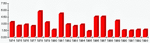
Frequently Asked Statistical Questions (INTERVENTION/OUTLIERS)QUESTION:I want to analyze whether there is a significant trend over time in the annual failure rate of a product. I have 20 years of measurements (i.e., n = 20). As I understand it, an ordinary regression analysis would be inappropriate because the residuals are not independent (i.e., the error associated with a failure rate for 1974 is more highly correlated with the 1975 failure rate than the 1994 failure rate). Is it appropriate to simply divide the data into two groups (the 1st 10 years vs. the 2nd 10 years) and do a between-groups ANOVA? Or is there some other (better) way to analyze these data? Should anyone be so inclined as to do the analysis, here are the data:
|
|
||||||||
|
Year |
Failure Rate |
|
||||||||
|
1974 |
3.3 |
|||||||||
|
1975 |
2.5 |
|||||||||
|
1976 |
2.7 |
|||||||||
|
1977 |
2.4 |
|||||||||
|
1978 |
5.7 |
|||||||||
|
1979 |
3.2 |
|||||||||
|
1980 |
1.6 |
|||||||||
|
1981 |
5.2 |
|||||||||
|
1982 |
2.8 |
|||||||||
|
1983 |
2.4 |
|||||||||
|
1984 |
2.7 |
|||||||||
|
1985 |
1.3 |
|||||||||
|
1986 |
4.5 |
|||||||||
|
1987 |
4.5 |
|||||||||
|
1988 |
1.4 |
|||||||||
|
1989 |
3.6 |
|||||||||
|
1990 |
1.5 |
|||||||||
|
1991 |
1.4 |
|||||||||
|
1992 |
1.6 |
|||||||||
|
1993 |
1.6 |
|||||||||
ANSWER:"The Heart of the Matter" Your question regarding "testing the differences between two means" where the breakpoint, if any, is unknown and to be found is an application of intervention detection. The problem can, and is in your case, compounded by unusual one-time only values. Another major complication, not in evidence in your problem, is the affect of autocorrelated errors and the need to account for that in computing the "t value or F value" for the test statistic. The answer to your question is 1. Don't assume that you need to break the data into two halves or some other guessed breakpoint. Employ Intervention Detection to search for that break point that provides the greatest distinction between the two developed groups. It is possible to pre-specify the test point, but it is clear from your question that you were just struggling. In some cases where the analyst knows of an event ( law change, regime change ) it is advisable to pre-specify, but most of the time this is a dangerous proposition as delays or lead effects may be in the data. 2. Adjusting for one time "onlies", analogous to Robust Regression, allows one to develop a gaussian process free of one-time anomalies and thus more correctly point to a break point. In this case:
|
|
|||||||||
|
OBSERVED VALUE |
TIME POINT |
ESTIMATED PULSE VALUE |
||||||||
|
5.7 |
1978 |
3.2 |
||||||||
|
5.2 |
1981 |
2.7 |
||||||||
|
4.5 |
1986 |
2.0 |
||||||||
|
4.5 |
1987 |
2.0 |
||||||||
|
3. After adjusting for these four "unusual values" the autocorrelation of the modified series exhibited the following;
|
||||||||||
|
LAG |
ACF VALUE |
STND. ERROR |
T- RATIO |
CHI-SQUARE |
PROBABILITY |
|||||
|
1 |
-.362 |
.224 |
-1.62 |
3.03 |
NA |
|||||
|
2 |
-.020 |
.251 |
-.08 |
3.04 |
NA |
|||||
|
3 |
.267 |
.251 |
1.06 |
4.88 |
NA |
|||||
|
4 |
-.329 |
.265 |
-1.24 |
7.86 |
NA |
|||||
|
5 |
.337 |
.285 |
1.18 |
11.18 |
NA |
|||||
|
6 |
-.297 |
.304 |
-.98 |
13.95 |
NA |
|||||
|
7 |
.032 |
.318 |
.10 |
13.99 |
.0002 |
|||||
|
8 |
.217 |
.318 |
.68 |
15.71 |
.0004 |
|||||
|
Analysis concludes that there is no evidence of any ARIMA structure. Note that if there was an ARIMA model, not some assumed model like Durbin's would be used to model the noise process for our generalized least squares estimator of the test for the significant difference between the two means of a specified or unspecified group size. Early reserachers in the 1950's (Durbin,Watson, Hildreth, Liu to name a few had to ASSUME the form of the error structure). More modern approaches skillfully IDENTIFY the form of the error process leading to correct model specification. Dated procedures should be treated very carefully as their simplicity can be your demise! One final comment, your question had to with things changing. It is possible that the mean might have changed or the trend might have changed. AUTOBOX speaks to both questions and in this case concluded that the mean had indeed changed. 3. In the final analysis, a "t test" is developed for the Hypothesis that
INPUT SERIES X5 I~AL0017 0017 LEVEL The conclusion based on a t value of -3.053, is that yes there is a
statistically significant difference between the two failure rates. This
conclusion is obvious when one looks at a plot. Click
here to view. |
||||||||||