A Modest Problem

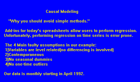
AFS has prepared a simple example of model building. This example has two series for some 54 monthly observations. To better understand AUTOBOX we suggest that you simply download the data and build a model using whatever tools you are comfortable with or have easy access to. You might even pass the data on to a colleague and get their input. The point is simply that you get more out of a presentation if you participate intellectually and develop a shared experience rather than simply watching or reading. To this end, we have prepared moddata.zip which contains the data. After you have done your "homework" the content of the following will be more appreciated and you can then return to the rest of this presentation. Statistics & Mathemathics are best learned by doing and reading.

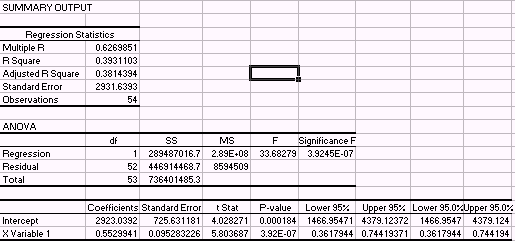
Perhaps some material on the subject of least squares. Gauss (1821) and Legendre (1806), both suggested the idea of minimizing squared deviations; Gauss pointed out 'But of all principles ours is the most simple; by others we would be led into the most complicated calculations'. Galton (1886) first used the term 'regression' in papers describing the relationship between the height of the children and of parents. We have seen generalizations of this to GLS models where the degree of importance of a certain set of x,y points is specified or developed as AUTOBOX does via the bootstrap. Extending regression to time series data has created issues such as latent variables and incorrect hypothesis testing. This particular example illustrates the opportunity to develop correct lag or model structures and to adequately deal with outliers and non-gaussian error processes.

ONE INPUT SERIES : INPUT.DAT

ONE OUTPUT SERIES : OUTPUT.DAT

MONTHLY DATA STARTING 1992/4

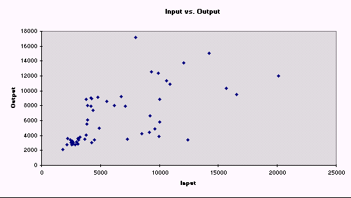
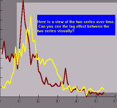
Consider the circumstance where monthly data is collected for 54 consecutive periods (1992/4 through 1995/9). We wish to develop a forecasting model that quantitatively relates these two series.

SCATTER PLOT OF INPUT VERSUS OUTPUT

PLOT OF INPUT AND OUTPUT VERSUS TIME NOTE: THE OUTPUT SERIES IS IN YELLOW NOTE: THE INPUT SERIES IS IN BROWN

NOTE THAT ORDINARY REGRESSION DOESN'T "SEE" THE LAGGED RELATIONSHIP AS THE MODEL THAT IS ESTIMATED IS SIMPLY CONTEMPORANEOUS (I.E. THE VALUE OF X AT TIME PERIOD "t" EFFECTS THE VALUE OF Y AT TIME PERIOD "t" AND ONLY AT THIS TIME PERIOD. Y(t) = 2923 + .55 * X (t)

ADVANTAGES OF SPREADSHEET TOOLS NEED TO BE LISTED. WHAT IS UNSAID OR UNSTATED ARE THE "ERRORS OF OMISSION" OR SIMPLY WHAT WAS NOT DONE THAT SHOULD HAVE BEEN DONE.

FOLLOWING IS A PLOT OF THE ACTUAL VERSUS THE MODEL FIT VALUES.

Examining Residuals For Structure After Taking Out The MEAN

WE NOW SYSTEMATICALLY EXPLORE THE PROCESS OF REDUCING DATA TO SIGNAL AND NOISE. DATA = SIGNAL + NOISE DATA IS THE OBSERVED SET SIGNAL IS WHAT IS EXPLAINED OR CONTRIBUTED BY THE MODEL & PARAMATERS NOISE IS THE UNEXPLAINED COMPONENT WE BEGIN BY BUILDING A MODEL BASED SIMPLY ON THE AVERAGE AND THEN WE INCREASE THE COMPLEXITY OF THE STRUCTURE OR SIGNAL. FOLLOWING IS A PLOT OF THE RESIDUALS FROM A MEAN MODEL Y(t)= CONSTANT + A(t)

Examining These Residuals for Structure After Taking out the EFECT OF THE MEAN

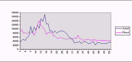
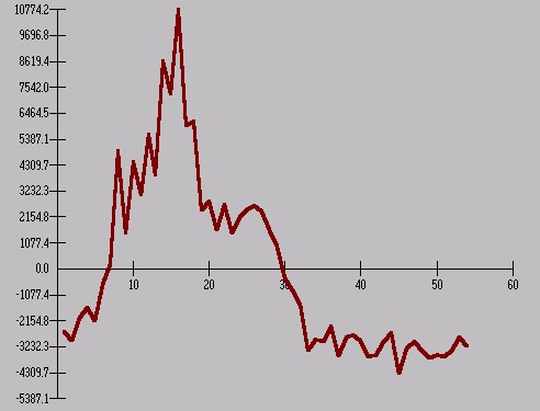
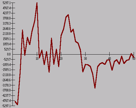
By plotting the residuals versus alternate lags of the input series it is possible to identify needed model augmentation strategies. Here we show the residuals and the input series lagged 0 periods illustrating the fact that the residuals can be predicted thus they are non-gaussian.

Examining These Residuals for Structure After Taking out Contemporaneous effect of Input

FOLLOWING IS A PLOT OF THE RESIDUALS FROM A MEAN MODEL + CONTEMPORANEOUS EFFECT OF INPUT Y(t)= CONSTANT W0 * X(t) + A(t)

Examining These Residuals for Structure

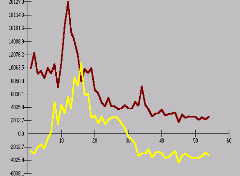
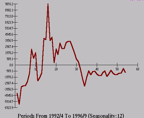
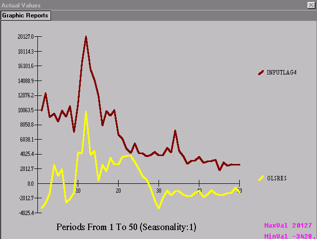
By plotting the residuals versus alternate lags of the input series it is possible to identify needed model augmentation strategies. Here we show the residuals and the input series lagged 4 periods illustrating the fact that the residuals can be predicted thus they are non-gaussian.

Examining Residuals For Structure After Taking Out The LAG 4 EFFECT

FOLLOWING IS A PLOT OF THE RESIDUALS FROM A MEAN MODEL + CONTEMPORANEOUS EFFECT OF INPUT + LAG 4 EFFECT OF INPUT Y(t)= CONSTANT W0 * X(t) + W1 * X(T-4) + A(t)

The residuals still exhibit a clear non-random structure as they would fail a visual "Run Test" which tests the sequence of positive and/or negative residuals. A trained "eye" can detect a number of violations in these residuals. Notice that the residuals tend to cluster around the mean. There are a bunch of positive residuals and then a bunch of negative reiduals followed by a bunch of positive residuals etc.. The residuals are thus predictable and fail the test. One way to deal with the issue is to use the Autocorrelation Function of the model residuals which suggested a first order autoregressive addition. This is auto-projective memory and in this case led to a model in first differences.

Examining Residuals For Structure After Taking Out The LAG 4 EFFECT AND FIRST DIFFERENCES AND THE AR LAG 2 EFFECT AND THE IDENTFIED INTERVENTIONS (OUTLIERS)

FOLLOWING IS A PLOT OF THE RESIDUALS FROM A MEAN MODEL + CONTEMPORANEOUS EFFECT OF INPUT + LAG 4 EFFECT OF INPUT + 2 IDENTIFIED INTERVENTIONS (1-B) Y(t)= CONSTANT W0 * (1-B) X(t) + W1 * (1-B) X(T-4) + A(t)/[1-PHI B] + W2 I1(t) + W3 I2(t)

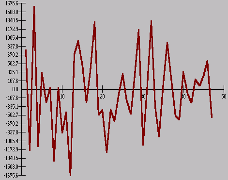
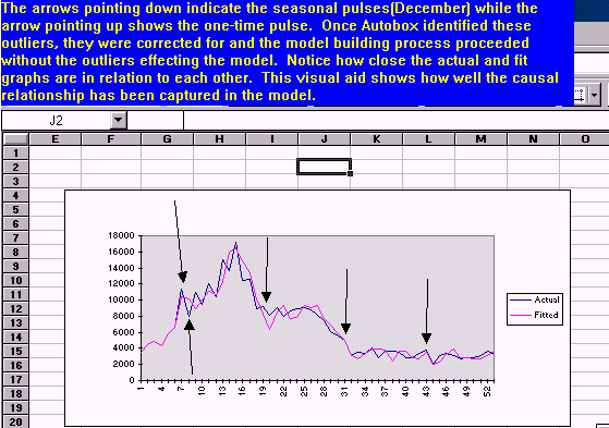
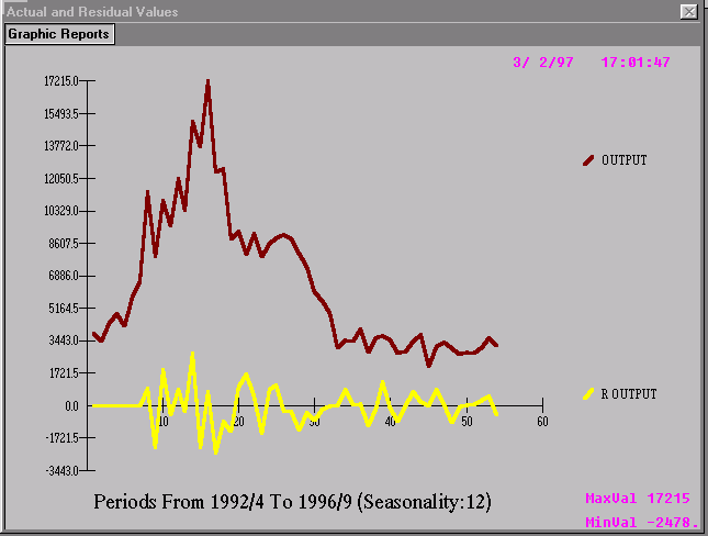
The residuals exhibit a clear random structure thus we can conclude the modelling process.

We now show the fit versus actual plot

We now show the actual and residual plot.

We now show the actual equation.

We now show the final model statistics.

We now show the final actual, fit and forecast plot

Click here to VIEW FULL ANALYSIS REPORT

Click here to go to SELF-DIRECTED TOUR

Click here to go to AFS SUGGESTED TOUR

Click here to return to the home page

P.O. Box 563
Hatboro, PA 19040
Tel: (215) 675-0652
Fax: (215) 672-2534
sales@autobox.com

CLICK HERE:Home Page For AUTOBOX