FORECASTING WEEKLY BEER SALES ... A CASE STUDY OF HOW
AUTOBOX IS CURRENTLY USED TO ANALYZE A HEAVILY PROMOTED PRODUCT. HURRY UP
AND JOIN THE PARTY !
THIS CASE STUDY DEVELOPS THE RELATIONSHIP OF PRICE AND VOLUME WHILE TAKING INTO ACCOUNT THE EFFECTS OF HOLIDAYS AND UNUSUAL ACTIVITY
ON WEEKLY BEER SALES.
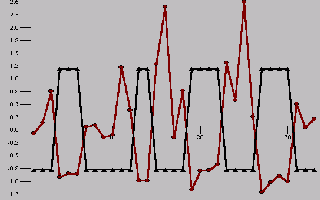
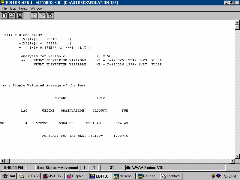
| When the distributor lowers his price, the customer reacts. This relocation of demand is a boon for forecasters and for statistical models as
the reaction is predictable and consistent. VOL SALES are in RED while PRICE is in BLACK. Note the persistence in the response of sales to price.
|  |
|---|
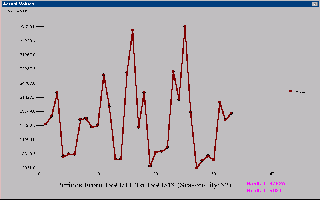
| Weekly beer sales for the period 1994/11 through 1994/43 illustrates
what the statistical problem is and what the business problem is. Consider
a simple approach to predicting this series and the implications.
|  |
|---|
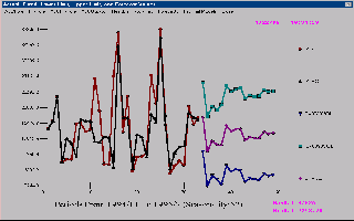
| The univariate, i.e. auto-projective model is based on the relationship
between successive observations. A four period relationship is identified and
used to make one period out predictions, the fit, and ultimately a forecast
for the next 16 periods ( week 44 through week 7 of 1995 )
|  |
|---|
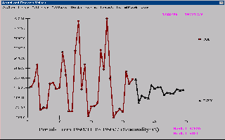
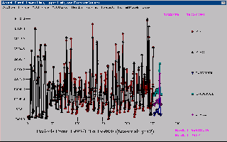
| Simplifying the graph, we have the historical values and the predicted values.
Note that the forecasts don't have the deep "swings" that the actual values
have and furthermore don't have the same "bunching together" appearance of
the actual historical values.
|  |
|---|
| Univariate models use the past of the series as a proxy for the omitted cause variable(s).
In this case, the genuine dissatisfaction with the forecast reflects the inadequacy
of a "rear-window" approach. One of the omitted variables is Price. Price is
a lever to create and to dislocate sales from one period to another. This
dislocation effect creates havoc for univariate modelers.
|  |
|---|
| An examination of an ARIMA model, reveals two unusual values or outliers. The
first unusual value occurs at week 35(8/29/94) while the second unusual value occurred at
week 26(6/27/94).
Note that the model identifies a negative response (inverse) to sales 4 weeks ago.
What this means is that if sales were high 4 weeks ago, current sales will be low.
The forecast equation is 21,742 multiplied by 57% of sales 4 weeks ago. Note
that the omitted variable Price has a 4 week profile.
|  |
|---|
| This equation arises because Price is varied in such a way that
sales increase with lower price (the low values are low price) and drop back when price is restored to its
normal level. The promotion calendar has a 4 week length thus the appearance
and inducement of a 4 period "seasonality". If sales were low, that is "off
promo" 4 weeks ago then sales will be high this week because we are "on promo".
|  |
|---|
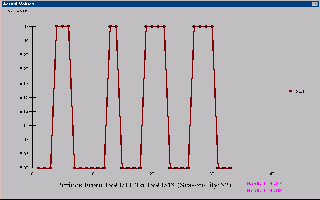
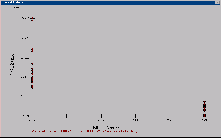
| The dependence of Sales on Price can be seen in a scatterplot showing
how Sales increase when the Price is low and Sales decrease at standard
pricing. Notice how all the points reflecting low price reflect high volume
while all the points for high price indicate low volume.
|  |
|---|
| The dependence of Sales on Price can be seen even clearer in this line
plot of VOL and PRICE against time ( 33 month period 1994/11 through 1994/43)
|  |
|---|
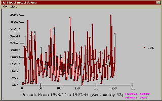
| We now will extend our model to include Price and some Holiday variables
to explain unusual and predictable "spikes" due to increase consumption around
Labor Day, July 4th , Memorial Day and of course St. Patrick's Day. We show here
sales for the period 1993/1 through 1997/44.
|  |
|---|
| First, we show Price on a weekly basis for the period. Notice that from
time to time major changes are made in the "Base Price" i.e. the nominal off
promo price.
|  |
|---|
| If we view both Sales and Price together the graph is somwehat busy do
to the length of the series. When we restricted ourselves to a 33 week period
the picture was very clear.
|  |
|---|
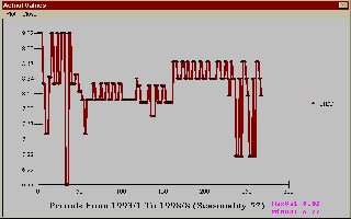
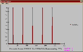
| We now show the July 4th Day variable.
|  |
|---|
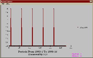
| We now show the Labor Day variable.
|  |
|---|
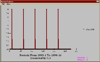
| We now show the Memorial Day variable.
|  |
|---|
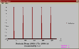
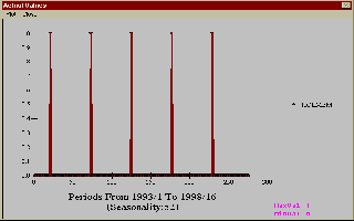
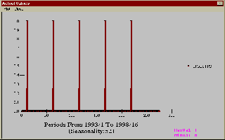
| We now show the first St. Patrick's Day variable. The St.Patrick's
Day effect was broken into three to refelect different responses depending
upon where it fell in the work week.
|  |
|---|
| We now show the second St. Patrick's Day variable.
|  |
|---|
| We now show the third St. Patrick's Day variable.
|  |
|---|
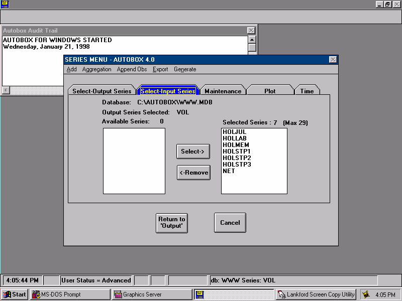
| We use AUTOBOX to select the input series that will be evaluated
in constructing a model for Sales.
|  |
|---|
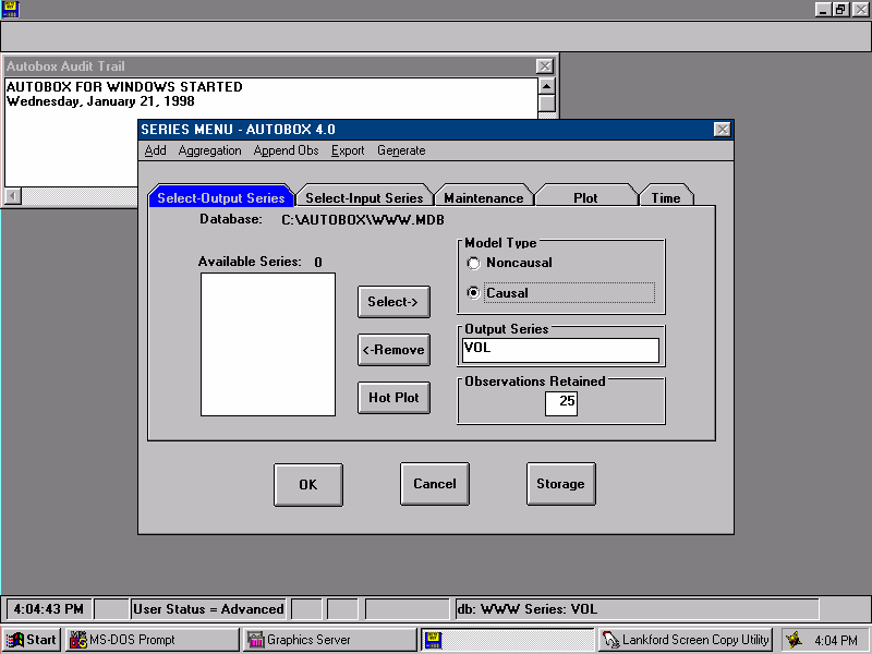
| We will withhold the most recent 25 values and prepare a 16 week ahead
forecast from each origin. Thus only one model and one set of parameters
will be developed. The forecast will be made and an assessment will be developed
measuring model performance.
|  |
|---|
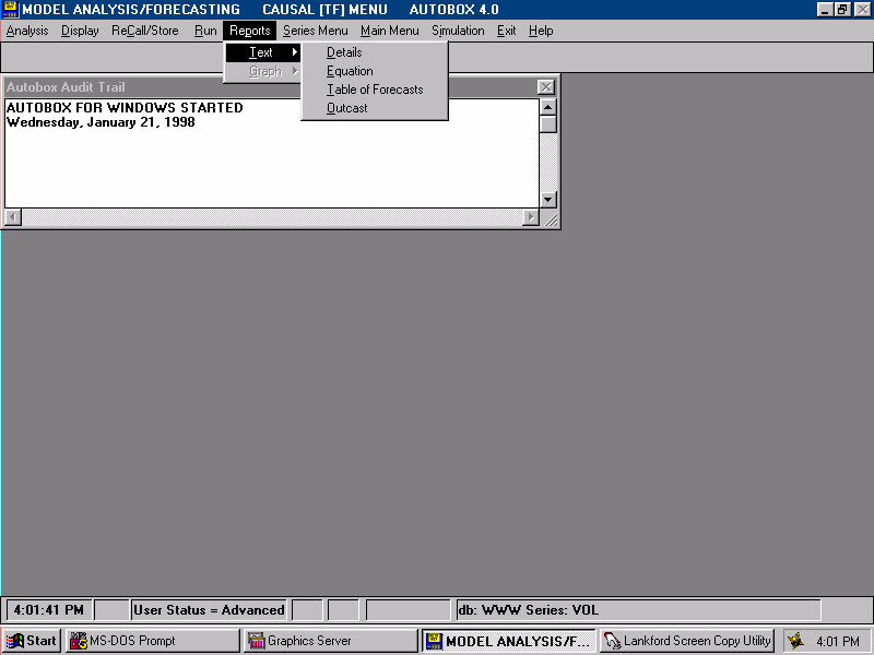
| After execution, we examine the "OUTCAST" analysis.
|  |
|---|
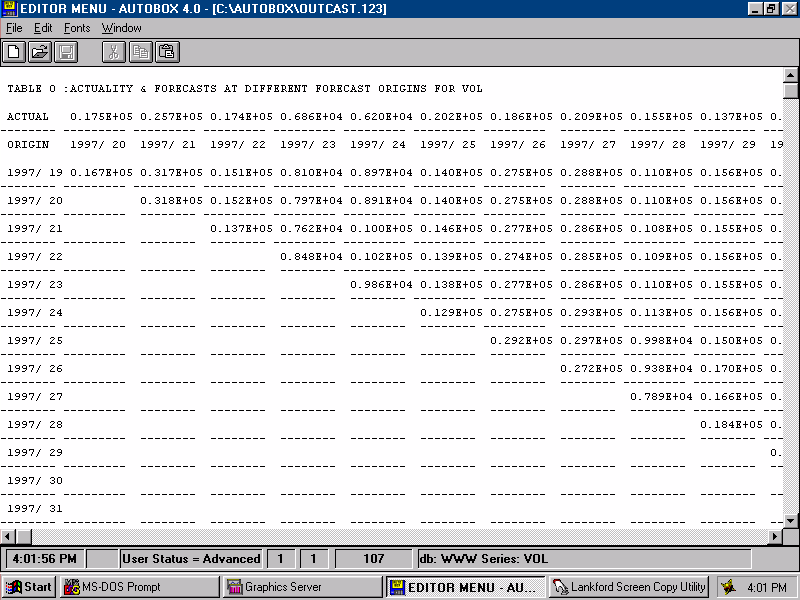
| The actual forecasts made from each origin are displayed.
|  |
|---|
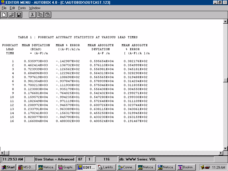
| A summarization of the forecast errors leads to TABLE 1.
|  |
|---|
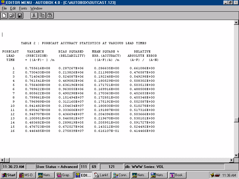
| A summarization of the forecast errors leads to TABLE 2.
|  |
|---|
| A side bar on measuring forecast accuracy
|  |
|---|
| Convinced that this approach was giving better forecasts than all
other known alternatives we remodel using all of the data. Here we show
the actual, fit and forecast.
the Plotcast option to view the results.
|  |
|---|
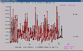
| Now just the actual and the forecasts are shown.
|  |
|---|
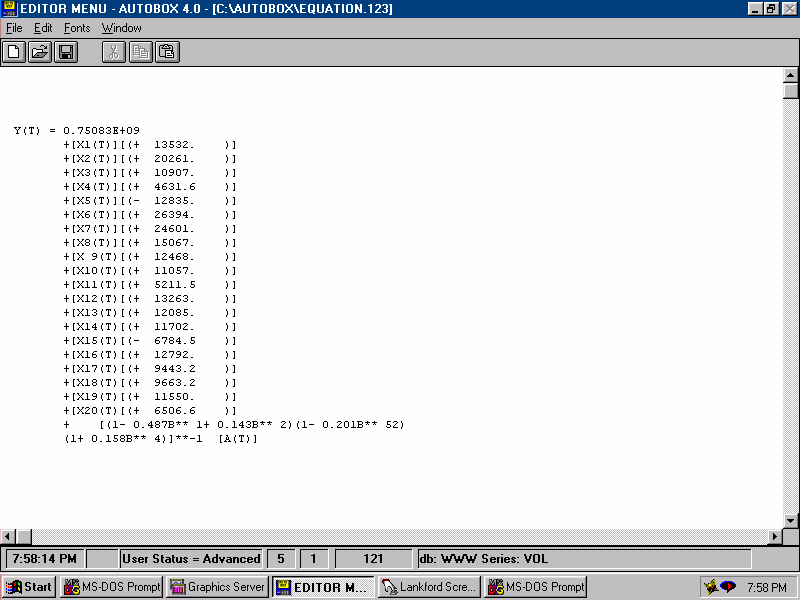
| Exploring the equation we find that the following variables were.
included in the final model.
|  |
|---|
| With coefficients ....
|  |
|---|
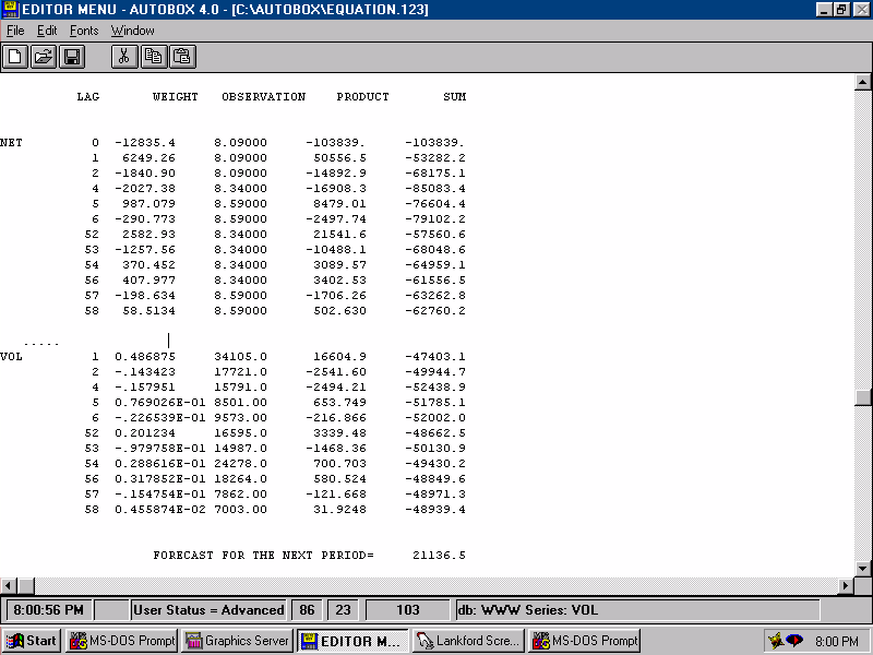
| As before the forecast is a weighted sum of the past and future values
of the input series.
|  |
|---|
|
The data.. HOLJUL,HOLLAB,HOLMEM,NET,VOL
|  |
|---|
CLICK HERE:Home Page For AUTOBOX
