Announcing the Option to run Autobox with where it will calculate Price elasticities automatically. Why is this so powerful?  If you have ever calculated a price elasticity, you might already know the modeling tradeoffs by using LOGS for a simplistic trick to quickly build the model to get the elasticity and the downside of doing so.  We aren't trading off anything here and using Autobox's power to do build a robust model automatically and considerig the impact of lags, autocorrelation and outliers.

We are rolling out an Option for Autobox 7.0 Command Line Batch to calculate "Short-Run" Price Elasticities.  The Price Elasticity Option can be purchased to produce Price elasticities automatically AND done the right way (we will explain that below) as opposed to assuming the model form to get a fast, but sub-standard econometric approach to calculating Price elasticities.  The Option allows you to specify what % change in price, specify the problems you want to run and then let Autobox run and model the data and produce a one period out forecast.  Autobox will run again on the same data, but this time using the change in price and generate another forecast and then calculate the elasticity with the supporting math used to calculate it stored in a report file for further use to prepare pricing strategy. That introduction is great, but now let's dive into the importance of modeling the data the right way and what this means for a more accurate calculation of elasticities! Click on the hyperlinks when you see them to follow the example.

For anyone who has calculated a price elasticity like this it was in your Econ101 class.   You may have then been introduced to the "LOG" based approach which is a clean and simple approach to modeling the data in order to do this calculation of elasticity as the coefficient will be the elasticity.  Life isn't that simple and with the simplicity there are some tradeoffs you may not be aware that came with this simplicity.  We like to explain these tradeoffs like this "closing the door, shutting the blinds, lowering the lights and doing voodoo modeling". Most of the examples you see in books and literally just about everywhere well intentioned analysts try and do their calculations using a simple Sales (Quantity) and Price model.  There typically is no concern for any other causals as it will complicate this simplistic world. Why didn't your analyst tell you about these tradeoffs?  You probably didn't ask.  If you did, the analyst would say to you in a Brooklyn accent "Hey, read a book!" as the books show it done this way. Analysts take LOGS of both variables and then can easily skip the steps needed in the first link above and calculate the elasticity, running a simple regression ignoring the impact of autocorrelation or other important causals and voila you have the elasticity which is simply found as the coefficient in the model.  The process is short and sweet and "convenient", but what happens when you have an outlier in the data?  What happens if you need to include a dummy variable?  What about the other causals? What about lags in the X?  What about autocorrelation? Does their impact just magically disappear? No.  No and no.

Let's review an example that Shazam uses from a text book to show how to model elasticity.  The "Canned Tuna" example comes from a textbook called "Learning and Practicing Econometrics" and it does try account for other causals so some credit is due here as most just use Price as the only causal.  We thought this was a good example to delve into as it actually tried to consider more complexities with dummies.  In the end, you will still want to forget everything you learned in that example and wish for a robust solution.  Here they only take LOGS of the Y variable as there are two causal dummy variables plus two competitor price variables.  They report the elasticity as -2.91%. They also do some kind of gyrations to get the elasticities of the dummies.   Now, we know that there is no precisely right answer when it comes to modeling unless we actually simulate the data from a model we specified. What we do know is that all models are wrong and some are useful per George Box.  With that said, the elasticity from a model with little effort to model the relationships in the data and robustitfied to outliers is too simple to be accurate.  Later on, we estimate an elasticity using the default of -2.41% but take no LOGS.  Is it that different?  Well, yes, it is. It is about 20% different.  Is that extra effort worth it? I think so. As for the model used in the text book and estimated in Shazam, the ACF/PACF of the residuals look well behaved and if you look at the t-values of the model everything is significant, but what about the residuals?  Are they random??? No.  The residual graph shows pattern in that it is not random at all.

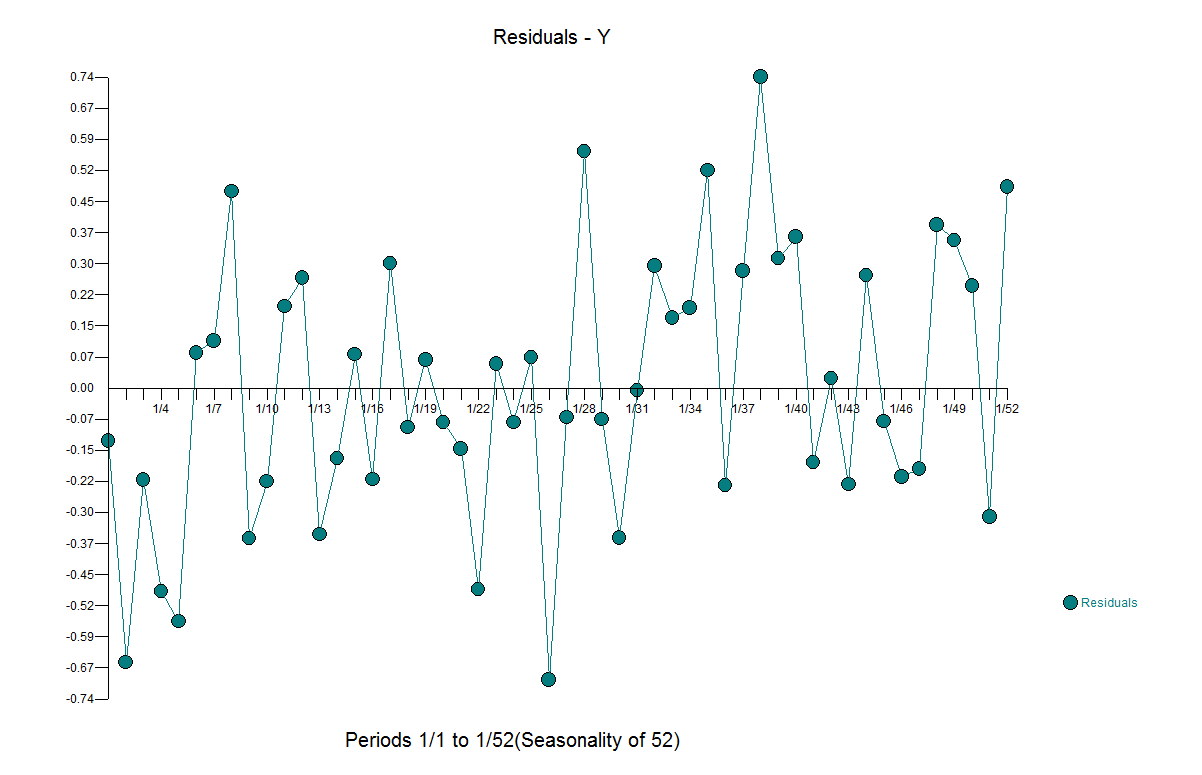
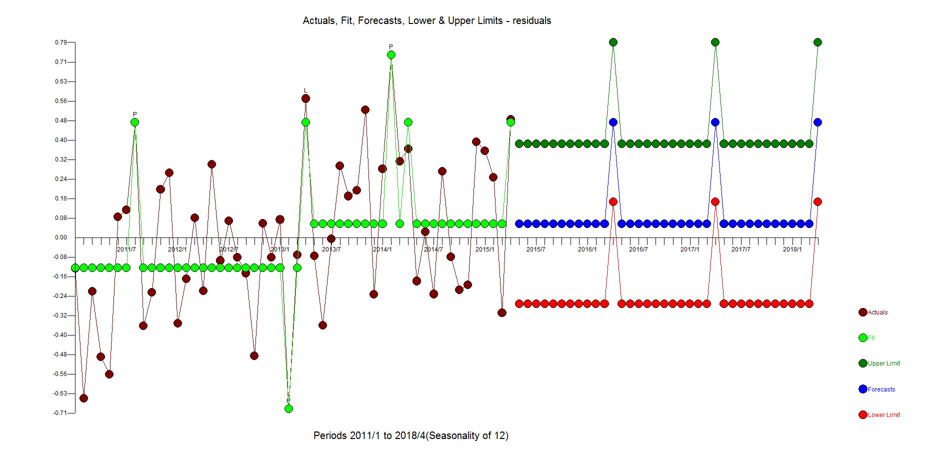
If you take the residuals and model them automatically in Autobox it finds a level shift suggesting that there is still pattern and that the model is insufficient and needs more care.

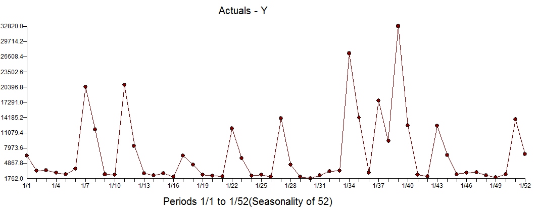
I would ask you to stop reading here and don't read the rest just yet.  I put a big graph of the history of Y right below so that your eyes won't see what's next.  Download the data set from the Shazam website and spend about 3 full days(and possibly nights) verifying their results and then building your own model using your tools to compare what Autobox did and of course questioning everything you were taught about Elasticities using LOGS. Feel free to poke holes in what we did. Maybe you see something in the data we don't or perhaps maybe Autobox will see something in the data you won't?  Either way, trying to do this automatically for 10,000 problem sets makes for a long non-automatic process.

 

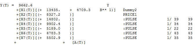
Let's not take LOGs and not consider any lags in the model or autocorrelation, but let's robustify the estimation of the Canned Tuna example by considering outliers, but let's NOT look for lags in the causals just yet. The signs in the model all make sense and the SOME outliers make sense as well(explained fully down below). It's not a bad model at all, but the elasticity is -5.51 and very far from what we think it should be. Comp1 and Comp2 is the competitor prices.

If we look at the ACF of the residuals, a small blip at 1 and 12 which really are not worth going after as they are marginal.

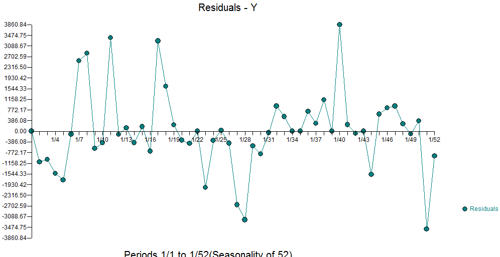
The residuals show what looks to be outliers.  While outlier detection was used, there are some things outliers can't fix.....bad modeling.

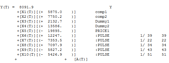
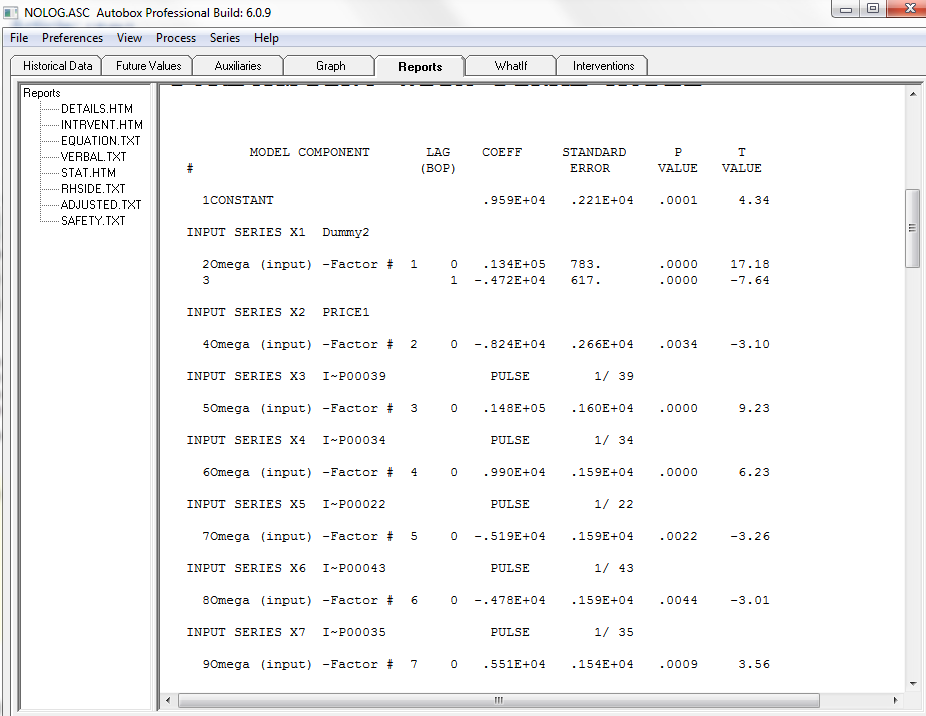
The issue with the Canned Tuna example is that there were variables being estimated and forced into the model aren't important at all and by including them in a "kitchen sink" type fashion they create "error" in the model specification bias and impacts the ability to accurately measure the elasticity plus not dealing with outliers.  Here are the Autobox results when you flag all of the causals to consider lag impacts(ie data_type=2).  It dropped three variables.  There was a lag impact which which was being ignored or really mismodeled by including the first dummy which has no explanatory power in the model.  There are some outliers identified.  Period 1/22 and 1/43 had an increase in sales, but those two promotions were much much lower than the others and are being adjusted up. In a similar fashion, the outliers found at 1/34, 1/35 and 1/39 were adjusted down as the promotions were way higher than they were typically. The elasticity calculated from the Autobox output is -2.41%.

Do the residuals look more random?  Yes.  Are there some outliers that still exist.  Well, yes but if you remove all the outliers you will have just the mean. You don't want to overfit.  You have to stop at some point as everything is an outlier compared to the mean.  Compare the size of these residuals with the graph above and this and the scale is much much smaller reflecting a better model.

 

Here are the model statistics.

 

Take a close look where dummy 1 was being promoted that week.  Take a look at weeks 1/2, 1/3, 1/9, 1/10, 1/24, 1/26, 1/36, 1/41, 1/42, 1/45, 1/46, 1/47, and 1/52.  None of them even did anything for sales.  Now there was one other area which could be debated at 1/17, 1/18 as having an impact, but just by eye it is clear that Dummy 1 is not a player.  What is clear is that Dummy 2 has an impact and that the week after it is still causing a positive impact.